Last lecture we traced WiFi’s twenty-year journey from distributed contention to centralized scheduling. We started with CSMA/CA and watched it succeed at low density, then crack under the overhead tax and the contention ceiling. We saw aggregation buy time, MU-MIMO crack the downlink, WiFox break fairness to save the AP [10], and 802.11ax finally centralize the MAC with OFDMA and Trigger Frames [3]. WiFi adopted distributed coordination not because unlicensed spectrum forced it, but for historical and practical reasons: Ethernet heritage (CSMA/CD adapted to half-duplex radio), the ad-hoc mode requirement (802.11 was designed for peer-to-peer operation), and low-complexity targets (the 1997 design assumed few devices, short-range indoor). Unlicensed spectrum imposes Listen Before Talk — spectral etiquette — but does NOT preclude centralized scheduling. Both 802.11ax and LTE-LAA prove that centralized scheduling works on unlicensed bands. The twenty-year delay in WiFi’s centralization was driven by deployment context and backward compatibility, not by a spectrum-imposed impossibility. Density eventually shifted the binding constraint until centralization became structural necessity, and WiFi ended up as a scheduled system.

Today we pick up the mirror image. Cellular never had to make that journey — because licensed spectrum grants one operator exclusive control over its band, so the base station was always the sole scheduler. No contention for discovery of who shares the channel; no need to evolve toward centralization. Cellular started where WiFi ended up — centralized from day one. Its evolution was a different question entirely: not when to centralize, but how to schedule efficiently as traffic changed from voice to data.

Licensed spectrum: the mirror binding constraint

WiFi’s original design context was unlicensed spectrum: no single entity has authority over the channel. This context, combined with Ethernet heritage and ad-hoc requirements, led to distributed Coordination, local State, coarse Time, and an Interface carrying minimal coordination information. But unlicensed spectrum does not architecturally preclude centralization — it requires Listen Before Talk (spectral etiquette), which is compatible with centralized scheduling as 802.11ax and LTE-LAA demonstrate.

Cellular’s binding constraint is the exact opposite. Licensed spectrum — exclusive operator ownership, purchased at auction for billions of dollars — locks Coordination to centralized from day one. One entity owns the channel. The base station is the sole authority over every transmission. There is no contention for data, ever. From this single fact, the invariant answers cascade in the opposite direction from WiFi:

• State can be global. The base station knows every registered device — its location, channel quality, traffic class, buffer status.
• Time can be precise. The base station synchronizes all transmissions to a global clock.
• Interface can carry rich scheduling information, because the base station controls both ends of every link.

So cellular’s story isn’t about escaping a coordination ceiling. It’s about an entirely different design challenge: how do you schedule a centralized channel efficiently when the nature of the traffic changes underneath you?

The measurement cost of centralized State

The statement “the BS knows every registered device” is true but hides a critical cost. Global state doesn’t materialize — it must be continuously measured, reported, and processed. The base station’s omniscience is purchased with airtime.

How the BS acquires global state:

• CQI (Channel Quality Indicator): The UE reports a summary of downlink SNR every TTI (1–2 ms). This tells the scheduler which modulation and coding scheme (MCS) to use for each user.
• CSI (Channel State Information): The full channel matrix needed for beamforming — includes PMI (Precoding Matrix Indicator) and RI (Rank Indicator). Far richer than CQI, far more expensive to report.
• SRS (Sounding Reference Signals): The UE transmits a predetermined pattern that both the UE and BS know in advance — like a test tone. Because the BS knows exactly what was sent, it can compare what it received against what was expected and compute how the channel distorted the signal (fading, phase shift, delay spread). This gives the BS a direct measurement of the uplink channel — essential for TDD systems where the BS uses uplink measurements to infer downlink channel conditions (reciprocity-based beamforming).
• DMRS/pilots: The BS transmits known symbols on the downlink so each UE can estimate its own channel and generate CQI/CSI reports.

The measurement tax:

In a massive MIMO configuration (320 MHz bandwidth, 16 antennas), CSI feedback per sounding event is approximately 22.4 KB, requiring ~7.5 ms to transmit at 24 Mbps. At a 10 ms sounding interval, this means roughly 75% of airtime is consumed by measurement overhead alone [13][15][16]. The scheduler’s global view is purchased at the cost of the very resource it is trying to schedule.

The Estimate–Measure–stale-By-the-time-you-use-it (E-M-B) paradox:

1. The wireless environment changes at coherence-time speed. Coherence time is the duration over which the channel’s characteristics (path loss, multipath reflections, fading) remain approximately constant — think of it as the “expiration date” on any channel measurement. It depends on how fast the transmitter, receiver, or reflectors are moving. At vehicular speeds (e.g., a car at 120 km/h on a 2 GHz carrier), coherence time is roughly 1.4 ms (see PHY Primer, Section 5 for the derivation from Doppler spread). At pedestrian speeds it stretches to tens of milliseconds; at stationary indoor positions it can be seconds.
2. Measurement takes time to generate (UE processing), compress (quantized CQI/PMI), transmit (uplink reporting), and process (scheduler computation).
3. By the time the scheduler uses a report, the channel may have changed. The scheduler allocates 256-QAM based on a stale “excellent” CQI report → the channel has faded → the transmission fails or requires retransmission.
4. Faster sounding reduces staleness but increases the measurement tax. Slower sounding reduces overhead but increases staleness. There is no escape from this tradeoff.

The fundamental coordination tradeoff:

	Distributed (CSMA/CA)	Centralized (scheduled)
Measurement	Local, binary (carrier sense)	Global, granular (CQI/CSI/SRS)
Overhead	Zero reporting; high collision risk	Massive reporting tax; zero collision
Failure mode	Contention collapse at density	Performance collapse from stale state

Distributed systems fail because they know too little — each station sees only its local carrier-sense observation, and at high density, that observation is insufficient to avoid collisions. Centralized systems can fail because maintaining what they know costs too much — the measurement overhead and staleness problem grows with the number of antennas, bandwidth, and user mobility. Neither architecture escapes the cost of coordination; they simply pay it in different currencies.

The cellular arc: FDMA, GSM, CDMA

First-generation cellular in the 1980s used Frequency Division Multiple Access (FDMA). The Advanced Mobile Phone System (AMPS), the dominant 1G standard in North America, operated in the 800 MHz band: 824–849 MHz uplink, 869–894 MHz downlink — 25 MHz in each direction, 50 MHz paired total. The FCC split this spectrum between two competing carriers per market (the A/B carrier split), giving each operator 12.5 MHz per direction. AMPS divided its allocation into 30 kHz channels, yielding 416 channels per operator in each direction (uplink and downlink). But frequency reuse — the practice of assigning the same frequencies to geographically separated cells to avoid interference — meant each individual cell had roughly 60 usable channels (Rappaport, Wireless Communications, 2002; Naik 2020). Capacity was hard: call number 61 was blocked outright, not degraded. And average voice activity is only about 35% — a speaker is silent roughly two-thirds of the time — so two-thirds of the allocated spectrum carried silence that nobody else could use. Hard allocation of a shared resource to bursty demand is structurally wasteful, but for voice circuits in the 1980s, simplicity was the binding constraint.

Spectrum evolution across cellular generations:

Gen	Band	BW per operator	Channel width
1G AMPS	800 MHz	25 MHz	30 kHz
2G GSM	900/1800 MHz	~25 MHz	200 kHz × 8 slots
3G UMTS	2100 MHz	~60 MHz	5 MHz wideband
4G LTE	700–2600 MHz	~100+ MHz	1.4–20 MHz, aggregatable
5G NR	3.5 GHz + 28 GHz mmWave	100–400+ MHz	Up to 100/400 MHz

The trend is unmistakable: each generation claims wider bands, higher frequencies, and more flexible channelization. The move from 25 MHz of fixed 30 kHz channels to hundreds of MHz of aggregatable resource blocks is the spectrum-domain expression of the same shift from hard to soft allocation that the MAC layer underwent (Naik 2020; 3GPP TS 36.300; 3GPP TS 38.300).

Second-generation GSM (Global System for Mobile Communications), deployed from 1991, switched from FDMA to Time Division Multiple Access (TDMA) [9]. Why the change? Digitization made it possible. AMPS used analog FM, which requires a continuous uninterrupted signal — you can’t time-slice an analog voice call. GSM digitized voice at 13 kbps, which meant voice could be buffered into discrete bursts and transmitted in time slots at a much higher burst rate (270.833 kbps) [9]. Eight users now shared one 200 kHz carrier, each getting a 576.9 microsecond slot within a 4.615 ms frame [9]. The effective bandwidth per user dropped from 30 kHz (AMPS) to 25 kHz (GSM), fitting more calls per MHz of operator spectrum. Hardware cost dropped too: FDMA needed one radio transceiver per active channel at the base station; TDMA shared one radio across eight slots [9]. Digital transmission also enabled encryption — impossible with analog FM. But GSM was still hard capacity: once all eight slots on all carriers were assigned, the next caller was rejected.

CDMA (Code Division Multiple Access), deployed commercially in the mid-1990s and the basis of all 3G systems, changed the paradigm entirely. The analogy: imagine a room where everyone speaks at the same time, but each pair of speakers uses a different language — one pair speaks English, another Japanese, another French [4]. If you understand English, the other languages don’t sound like speech to you; they just sound like low-level background murmur. As long as that murmur isn’t too loud, you can follow your own conversation perfectly.

Mechanically, CDMA maps to three CS concepts you already know:

• XOR encoding. Each user’s data bit is multiplied by a unique high-rate spreading code — functionally identical to XORing a bitstream with a pseudo-random key [4]. The 802.11 standard uses the same XOR scrambling logic for synchronization [2]. All users transmit their encoded signals simultaneously on the same frequency. At the receiver, the incoming signal — a sum of everyone’s encoded transmissions — is multiplied (XOR’d) by the intended user’s code. Original data bit pops out.

• Hash independence. The codes are orthogonal — their dot product is zero, like hash functions mapping to non-colliding buckets [4]. Multiplying by a different user’s code produces a result that averages to zero. If you know the key, you decode the data. If you don’t, it looks like random noise.

• Error-correction redundancy. Each data bit is spread across many chips — where a chip is one element of the spreading code, transmitted at 1/128th the duration of the original data bit. If your data rate is 9.6 kbps, and you spread each bit across 128 chips, you’re transmitting chips at 1.2288 Mchips/sec — using 128× more bandwidth than the data strictly requires [4]. Why pay that cost? Because spreading gives the receiver processing gain: the ratio of chip rate to data rate (128, or about 21 dB). The receiver can suppress interference up to 128× stronger than the desired signal by averaging across all 128 chips — the same logic as adding redundant parity bits in error-correction codes. But only up to that limit. Beyond it, the math breaks and bits are lost.

(For more detail on how this maps to the physical layer, see the Wireless PHY Primer.)

Why adding a user raises the noise floor — the key step.

In FDMA, each user gets a private frequency slot. If user A is on 870.030 MHz and user B is on 870.060 MHz, user A’s receiver simply ignores 870.060 MHz. The signals are physically separated — one user’s transmission does not appear in another user’s receiver at all.

CDMA is fundamentally different. All users transmit on the same frequency, at the same time [4]. The base station receiver hears a single composite signal — the arithmetic sum of every user’s encoded transmission. The codes let the receiver mathematically extract one user’s data from that sum (despreading). But the other users’ signals don’t vanish — they remain in the composite as residual energy.

Return to the cocktail party. With 3 people speaking 3 languages, the background murmur is faint — you follow your conversation easily. With 30 people, the room is louder. With 100, you’re straining to hear. Each additional speaker adds volume to the room, even if they’re speaking a language you don’t understand. The languages (codes) haven’t changed — they’re still mutually unintelligible — but the total acoustic energy in the room has increased. At some point the murmur overwhelms your ability to pick out your partner’s voice.

Quantitatively: the processing gain (128× in CDMA voice) is the receiver’s ability to suppress interference from each other user. But each user contributes some residual interference that the processing gain cannot fully cancel — especially because in practice, multipath reflections cause signals to arrive with slight time delays, which breaks the perfect orthogonality of the codes [4]. The total interference from $n-1$ other users must stay below the processing gain threshold. Gilhousen et al. [4] derived that the capacity of a CDMA cell is approximately:

\[N \approx \frac{W/R}{E_b/N_0} \times \frac{1}{1 + f} \times \text{(voice activity factor)}\]

where $W/R$ is the processing gain (128), $E_b/N_0$ is the minimum signal-to-noise ratio the receiver needs to decode reliably (about 7 dB for CDMA voice), and $f$ is the ratio of out-of-cell to in-cell interference [4]. The capacity is interference-limited, not channel-limited. There is no hard wall — no “channel 61 is blocked.” Instead, each new user degrades every existing user’s signal quality by a small, measurable amount. This is soft capacity instead of hard capacity.

But soft capacity creates a critical vulnerability: power.

Imagine the cocktail party again. If one speaker shouts at 100× normal volume, it doesn’t matter that they’re speaking a different language — the sheer volume drowns out every other conversation in the room. This is the near-far problem: a mobile phone 100 meters from the base station arrives at the receiver approximately 10,000 times stronger (40 dB) than one a kilometer away, completely masking the distant user [5]. The “orthogonal languages” only work when everyone speaks at roughly the same volume.

The fix: the base station commands each mobile to adjust its transmit power 800 times per second [5], keeping all signals arriving at roughly equal strength. This closed-loop power control IS the medium access mechanism in CDMA — not backoff, not scheduling, but continuous real-time power management. If one user’s power control loop fails or lags, that user’s signal drowns everyone else’s. The system’s capacity is literally the sum of interference from all users; managing that interference in real time is the MAC [4][5].

The soft-capacity model was the conceptual precursor to packet-switched data scheduling. If resources can be shared dynamically — rather than allocated in fixed blocks that sit idle during silence — then you can match allocation to demand on short timescales. CDMA proved that dynamic sharing works at millisecond granularity. But all three systems — FDMA, TDMA, CDMA — were designed for voice: steady, symmetric, circuit-switched traffic well-served by dedicated channels.

From voice to data: progressive disaggregation

In Chapter 1 we introduced disaggregation as a design principle: separating coupled concerns into independently controllable dimensions. The canonical example was the Internet protocol stack — DNS separates naming from addressing, TCP separates reliable delivery from routing, each layer can evolve independently. We also noted the cost: every separation boundary introduces a coordination signal, and that signal can degrade. The layered stack forces TCP to infer congestion because IP’s interface hides router queue state.

But what is the cost of NOT disaggregating? What happens when you leave coupled concerns fused in a monolith? The cellular RAN from 1991 to 2009 is a case study in paying that cost — and being forced, generation by generation, to separate things that should never have been joined.

The monolith: GSM’s base station.

GSM’s BTS (Base Transceiver Station) was a single vertically-integrated cabinet. Radio hardware, baseband DSP, and control logic — all from one vendor, all in one box. Above it sat the BSC (Base Station Controller), which managed multiple BTSs and made all resource allocation decisions. Above that, the MSC (Mobile Switching Center) handled call routing and billing. Three tiers, each proprietary, each from the same vendor.

For voice, this monolith made sense. The service was uniform: 13 kbps codec, symmetric, circuit-switched, calls lasting minutes. The “scheduling” problem was trivial: assign a TDMA slot per call, hold it for the duration. Nothing inside the system needed to change on millisecond timescales. The cost of NOT disaggregating was zero — because nothing needed to evolve independently.

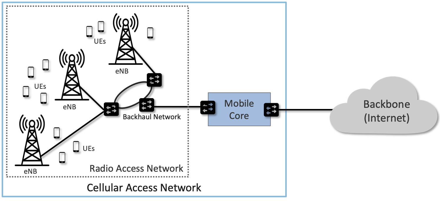
Terminology note: Every cellular generation renamed the same physical thing — the equipment at the cell tower. GSM called it the BTS (Base Transceiver Station). 3G called it the NodeB. 4G called it the eNodeB (eNB). 5G calls it the gNodeB (gNB). They all do the same fundamental job: connect mobile devices (UEs — User Equipment) to the network. What changes across generations is the boundary of what’s inside that box — and that shifting boundary IS the disaggregation story.

The first cost: 3G and the RNC bottleneck.

UMTS (3G) inherited this monolithic thinking. The architecture had three layers: the NodeB (the base station — radio hardware + baseband, but “dumb” — it didn’t make scheduling decisions), the RNC (Radio Network Controller — a separate box that made ALL scheduling, handover, and resource management decisions), and the core network [6]. The RNC sat physically separate from the NodeBs, connected via the Iub interface. One RNC controlled dozens of NodeBs.

What happens when traffic changes from voice to data? Voice is steady — a phone call occupies its channel for minutes at roughly constant bit rate. Data is bursty — loading a webpage involves a few hundred milliseconds of intense transfer, then seconds of idle reading. Under the circuit model, you hold a dedicated channel the entire time. The utilization is terrible.

The fix is obvious: schedule dynamically, giving the shared resource to whoever needs it NOW. But the RNC made all scheduling decisions. The round-trip signaling delay on the Iub interface was 10–20 ms. For voice circuits this was fine — a call lasts minutes. For packet scheduling it was fatal. Channel conditions change every 1–2 ms. By the time the RNC’s decision reaches the NodeB, the channel has faded and the decision is stale.

This is the cost of not disaggregating. The scheduling function and the channel-measurement function were separated by an interface that imposed 10–20 ms of latency — not because they needed to be separate, but because the 1991 architecture fused “radio resource decisions” into a single remote controller without distinguishing which decisions were time-critical and which were not. Handover decisions (which base station should serve this user?) tolerate 100 ms of delay. Scheduling decisions (which user gets this TTI?) cannot tolerate 10 ms. But the monolithic RNC handled both, at the same location, with the same interface latency.

Clarification: MAC vs. scheduler.

Students often ask: are “MAC” and “scheduling” the same thing? In WiFi, they effectively are — CSMA/CA IS the medium access mechanism, and there is no separate scheduler. The MAC layer and the access decision are fused into one distributed protocol.

In cellular, the MAC is a broader protocol layer that handles several jobs besides scheduling [7]:

• Retransmission — if a transmission fails (the receiver couldn’t decode it), the MAC decides whether to resend the same data or send additional error-correction bits. This is HARQ (Hybrid Automatic Repeat Request) — the same ACK/retry logic you know from TCP, but operating per-frame at millisecond timescales instead of per-segment at RTT timescales.
• Framing — the MAC packages higher-layer data (IP packets, signaling messages) into transport blocks sized to fit the current radio conditions. Think of it as fragmentation and reassembly — the same problem TCP solves with MSS, but adapted to a channel whose capacity changes every millisecond.
• Random access — handling the RACH procedure we discussed above, where new devices announce themselves via contention.
• The scheduler — the decision engine that answers “who gets which resource blocks this TTI?” This is the most consequential MAC function, but not the only one.

When we say “HSDPA moved the scheduler into the NodeB,” we mean specifically the resource-allocation decision. The other MAC functions (retransmission, framing) already lived at the NodeB — they had to, since they operate at frame timescales. The scheduler was the outlier: the one time-critical function stranded at the wrong location.

First disaggregation: HSDPA splits the RNC along the time axis.

High Speed Downlink Packet Access (HSDPA), specified in 3GPP Release 5 and deployed commercially around 2005, was not just a speed upgrade — it was a disaggregation event [6]. HSDPA kept CDMA’s air interface but moved the packet scheduler out of the RNC and into the NodeB itself. The RNC retained slow-timescale functions (handover decisions, radio bearer setup, connection management). The fast-timescale function — who transmits in this 2 ms TTI — moved to where the channel information lived.

This is the decision placement principle from Chapter 1: put decisions where the information lives. The scheduler needs per-millisecond channel state; channel state lives at the NodeB; therefore the scheduler must live at the NodeB. The RNC’s 10–20 ms control loop was structurally incapable of sub-millisecond scheduling. Moving the function was forced by the Time invariant.

Think of TTI (Transmission Time Interval) as the cellular answer to the Time invariant: how often does the scheduler re-evaluate? Every 2 ms, the scheduler observes the channel conditions of all active users — reported via CQI (Channel Quality Indicator) feedback, the cellular answer to the State invariant — and gives the shared pool’s resources to the users who can use them best right now.

Opportunistic scheduling — the payoff of disaggregation. Instead of assigning a fixed channel to each user (who mostly wastes it), give the shared resource to whoever has the best channel conditions at this instant. A user experiencing a temporary signal peak gets the resources; a user in a fade waits for conditions to improve. The aggregate throughput increases because the system rides the peaks of each user’s channel. This was impossible when scheduling lived at the RNC. The cost of the old monolith was not just latency — it was the inability to implement an entire class of algorithms.

Second disaggregation: LTE eliminates the RNC.

HSDPA proved per-TTI scheduling works. But it was a patch — the RNC still existed, still controlled handovers, still added cost and latency for every control-plane operation. LTE (Long Term Evolution, 3GPP Release 8, deployed 2009) took the lesson further: eliminate the RNC entirely [7].

The eNodeB (eNB) absorbed ALL radio resource management functions — scheduling, handover execution, radio bearer management, interference coordination. The architecture flattened from three tiers (NodeB → RNC → Core) to two (eNB → Core). A new direct interface, X2, connected neighboring eNodeBs for handover coordination — peer-to-peer, without passing through any centralized controller [7].

What did this enable for the MAC? With the scheduler co-located in the eNB and no RNC bottleneck, LTE built its entire air interface around OFDMA — dividing the channel into time-frequency resource blocks and scheduling them every 1 ms TTI [7]. The scheduler could react to per-user, per-subband channel quality at millisecond granularity. OFDMA was not just a PHY technique — it was architecturally enabled by the disaggregation that put the scheduler in the right place. This is the same OFDMA that WiFi would borrow in 802.11ax twelve years later.

Third disaggregation: LTE splits the core.

Simultaneously, LTE disaggregated the core network along a different seam: control plane vs. user plane. The MME (Mobility Management Entity) handled signaling — authentication, session setup, handover orchestration. The S-GW and P-GW handled data forwarding. These could now scale independently: more users = more MME signaling capacity; more traffic = more gateway forwarding capacity. The circuit-switched voice core (MSC) was deprecated — voice became just another IP flow (VoLTE) [7].

The progressive pattern.

Generation	What was monolithic	What got disaggregated	Why	What it enabled
GSM (1991)	Everything	Nothing	Voice was uniform — no reason to split	Simple, cheap, worked
3G/HSDPA (2005)	RNC = slow decisions + fast decisions	Scheduler → NodeB	Data scheduling needs ms timescales; Iub imposed 10–20 ms	Opportunistic scheduling, 2 ms TTI
4G/LTE (2009)	RNC = handovers + bearer mgmt	RNC eliminated; eNB absorbs all	RNC added cost/latency with no remaining benefit	1 ms TTI, OFDMA, X2 peer coordination
4G core	Core = signaling + forwarding	MME (control) / S-GW+P-GW (data)	Independent scaling; deprecate circuit voice	VoLTE, elastic data plane
5G (next lecture)	eNB = RF + baseband + control	CU / DU / RU along timescale boundaries	Pooling, edge compute, multi-vendor	Programmable scheduling, O-RAN

Each row is forced by the same logic: a function that needs to operate at timescale X cannot live behind an interface that imposes latency > X. When the environment changes (voice → data → diverse services), the timescale requirements diverge, and the monolith must split along those diverging seams. The cost of NOT splitting is that the fastest function is throttled to the speed of the slowest interface.

Connecting back to Chapter 1. The book said: “The cost [of disaggregation] is interface overhead. Every separation boundary introduces a coordination signal.” True — the X2 interface between eNodeBs introduces signaling that the old RNC handled implicitly. But the cost of NOT disaggregating is worse: it locks the system’s evolution speed to its slowest component. The RNC could not evolve scheduling algorithms independently of handover logic. The monolithic eNB cannot evolve its radio without changing its scheduler. Each disaggregation event unlocks independent evolution of the separated components — exactly what the Internet protocol stack achieved for naming, addressing, and routing.

In L9, we will see 5G crack open the eNB itself — separating microsecond functions (RF, beamforming → RU) from millisecond functions (scheduling, HARQ → DU) from tens-of-milliseconds functions (RRC, mobility → CU). The lesson is not “disaggregate everything from the start.” It is: disaggregation is forced when the system’s environment changes and its components need to evolve at different speeds. You don’t pay the interface cost until you need the independence. GSM didn’t need it. LTE did. 5G needs even more.

The universal bootstrap: RACH

Here is one of the most satisfying observations in the entire wireless landscape.

GSM is a fully centralized system — zero contention for data. The base station schedules every transmission. But there is one moment when centralization fails: when a brand-new device powers on. The base station doesn’t know it exists. It cannot schedule what it has not discovered. So the device announces itself in a special slot called the Random Access Channel (RACH) — using slotted ALOHA [9]. The 1972 protocol, running inside a 1991 TDMA system.

The mobile transmits a short access burst in a designated RACH slot, hoping no other mobile picked the same slot at the same time. If two mobiles collide, they back off a random interval and retry. This is literally slotted ALOHA — the same protocol we studied in L5.

Could you eliminate RACH entirely? Could you build a system with zero contention at every level? No. Any system with dynamic membership — where new participants can join without prior arrangement — needs at least one contention-based moment: the discovery moment. You can centralize everything after discovery, but discovery itself is irreducibly contention-based. There is no way for the base station to schedule a device it doesn’t yet know about. The device must announce itself, and multiple devices might announce simultaneously. Contention is the tax you pay for letting new participants join.

802.11ax has exactly the same pattern: OFDMA for data (centralized scheduling, zero contention), CSMA/CA for initial association (contention-based discovery). Two systems that started from opposite ends of the spectrum — one fully distributed, one fully centralized — both retain contention for exactly one purpose: bootstrap.

The unifying lens: feedback loop speed

Every wireless MAC, whether distributed or centralized, is fundamentally a control loop: measure the channel, allocate resources, transmit, measure the outcome, reallocate. The speed of that loop — how fast the system can observe conditions and react — determines the architecture’s ceiling. This is distinct from the overhead tax we studied in L7, which is about how much airtime each individual frame attempt wastes. Loop speed is about how quickly the system adapts to changing conditions across all users.

But as we saw in the measurement-cost section above, a faster loop is only half the story. The loop runs faster in centralized systems, but maintaining the global state that feeds it is expensive — CQI/CSI/SRS reporting consumes airtime, and the reports can go stale before the scheduler acts on them. The table below shows the loop getting faster from left to right; keep in mind that the rightmost entries also carry the heaviest measurement tax.

System	What it measures	Loop period	Coordination
CSMA/CA	Carrier sense (local, binary: busy or idle)	~12 ms	Distributed
GSM TDMA	Slot assignment (fixed per frame)	~4.6 ms	Centralized
CDMA power control	Received power per user	~1.25 ms (800 Hz) [5]	Centralized
LTE OFDMA	CQI per user per resource block	~1 ms [7]	Centralized
802.11ax OFDMA	Per-client channel feedback	~1-5 ms	Centralized

The pattern is clear: faster loop, tighter coordination, higher utilization. CSMA/CA had the slowest loop in the entire landscape. It measures locally — carrier sense at the transmitter, a binary observation — and gets feedback only after the full frame exchange completes (ACK or timeout). At legacy 1 Mbps rates, that loop period is roughly 12 milliseconds.

GSM’s TDMA loop runs at 4.615 ms frame periods. CDMA’s power control loop runs at 800 Hz — every 1.25 milliseconds, fast enough to track vehicular Rayleigh fading. Rayleigh fading is the rapid fluctuation in received signal strength caused by multipath reflections arriving at slightly different times and constructively or destructively interfering — a car moving at highway speed experiences signal peaks and nulls on the order of milliseconds (see PHY Primer, Section 5). LTE measures CQI reports and reallocates resource blocks every 1 ms TTI. 802.11ax operates at comparable timescales with Trigger Frames.

CSMA/CA suffers a double penalty: it has both the highest overhead tax (160 microseconds of protocol gaps per frame, regardless of PHY rate) [1][2] and the slowest feedback loop. That combination is the structural reason contention broke under density — and why centralization, with its faster and richer feedback, was the destination for both WiFi and cellular. But centralization’s faster loop comes with its own cost: the measurement tax and staleness problem we analyzed earlier. The convergence story is not “centralization wins” — it is “centralization trades collision overhead for measurement overhead, and at scale, the measurement tradeoff is better.”

Convergence: each side borrowed the other’s technique

After thirty years of divergence, WiFi and cellular arrived at the same architecture. The convergence happened from both directions.

WiFi started fully distributed. It fought through twenty years of PHY improvements — OFDM, MIMO, wider channels, higher-order modulation — and MAC patches — aggregation, Block ACK, TXOP — trying to escape the contention ceiling without changing the binding constraint. When density finally shifted the constraint from “no authority over spectrum” to “coordination cost exceeds capacity,” WiFi centralized. 802.11ax borrowed OFDMA from LTE [3]. The AP became a scheduler.

Cellular started centralized from day one. But in 2016, when cellular operators wanted to supplement their licensed spectrum with unlicensed 5 GHz bands, they faced a problem WiFi had always lived with: other devices were already transmitting in that spectrum, and the cellular base station couldn’t schedule them. It couldn’t assert authority over spectrum it didn’t own. So 3GPP Release 13 specified Licensed-Assisted Access (LAA), which required LTE to adopt Listen Before Talk (LBT) — carrier sensing, the core WiFi mechanism — before transmitting in unlicensed bands [8]. Cellular had to learn contention because the spectrum constraint demanded it.

Each side borrowed the other’s core technique for the exact reason the other side had adopted it originally. WiFi borrowed centralized scheduling because density demanded it. Cellular borrowed distributed contention because shared spectrum demanded it. The framework predicts this: identical constraints force identical invariant answers, regardless of starting point [11].

And both retain contention for exactly one purpose: bootstrap. Cellular uses RACH for device discovery. WiFi retains CSMA/CA for initial association. The universal architecture is: schedule everything you can, contend only for discovery.

The destination was determined by physics and density. The path depended on where you started.

In-class exercise: when one queue serves three masters

In L7 you computed τ and P(success) and watched CSMA/CA collapse under density — same formula, same result whether it’s a stadium or a warehouse. Today’s exercise holds density fixed and changes what breaks: not the number of devices, but the diversity of what they need.

Setup. A hospital wing runs all wireless traffic through a single 802.11ac AP on a 80 MHz channel. Three device classes share the channel:

1. 20 patient monitors — each sends a 200-byte vitals packet once per second (heart rate, SpO₂, blood pressure). Tolerance: delivery within 500 ms is fine; a 2-second delay triggers a nuisance alarm but is not dangerous.
2. 5 staff tablets — intermittent video consultations and image pulls. Bursty: 2 Mbps when active, idle most of the time. Tolerance: 50–100 ms latency is acceptable; buffering is annoying but not harmful.
3. 1 surgical telerobotic console — continuous haptic feedback loop between surgeon and remote instrument. 500 Kbps bidirectional, continuous. Tolerance: if any single packet exceeds 10 ms one-way delay, the surgeon feels a control discontinuity; above 50 ms, the procedure must pause.

Total station count: $n = 26$. Not a stadium. Not even a crowded café.

Part 1 — Does CSMA/CA collapse here?

Apply the formula from L7: $\tau = 2/(CW_{\min} + 1) = 0.125$, $P(\text{success}) = n \cdot \tau \cdot (1-\tau)^{n-1}$.

At $n = 26$: $P(\text{success}) = 26 \times 0.125 \times (0.875)^{25} = 3.25 \times 0.0325 \approx 0.106$.

About 10% of slots succeed. Not catastrophic — not zero like the stadium. CSMA/CA is degraded but functional. Throughput exists. So density is not the problem here.

Part 2 — What IS the problem?

CSMA/CA treats every frame identically. The surgical console’s haptic packet enters the same contention queue as a monitor’s vitals reading and a tablet’s video chunk. There is no priority, no deadline awareness, no isolation.

Ask students: What is the worst case the surgical console faces?

• A tablet initiating a large image transfer wins the channel and transmits for one TXOP (up to 5.484 ms in 802.11ac). The haptic packet waits.
• Multiple monitors happen to transmit in the same slot → collision → everyone backs off → the haptic packet’s backoff counter hasn’t reached zero yet.
• The haptic packet finally wins after 3 backoff rounds. Each collision doubles CW. Average backoff at CW = 63 is ~31 slots × 9 µs = 279 µs per round, plus DIFS (34 µs) each time. Three rounds: ~1 ms of backoff alone, plus the time waiting for the channel to go idle between each attempt.
• Total delay: TXOP wait + backoff + transmission ≈ 5–8 ms in a moderate scenario. Under load spikes (multiple tablets active simultaneously), 10–15 ms is realistic.

The 10 ms deadline is not reliably met — not because the channel is saturated, but because the MAC has no concept of urgency. A 200-byte heartbeat reading and a 10 ms-critical haptic command are indistinguishable to the backoff counter.

Part 3 — Could OFDMA fix this?

With 802.11ax OFDMA on an 80 MHz channel: 37 RUs available (each 26 subcarriers ≈ 2 MHz). The AP could reserve:

• 1 RU permanently for the surgical console — dedicated, contention-free, guaranteed every Trigger Frame
• 5 RUs for tablets when active, released when idle
• Remaining RUs shared among monitors via scheduled polling

The surgical console gets deterministic access every scheduling cycle (~1–5 ms). No contention, no backoff, no waiting behind a tablet’s video burst. The 10 ms deadline is met structurally.

But notice what the AP must now do: it must know that the surgical console needs 1 RU every millisecond, that the tablets are bursty, and that the monitors can tolerate 500 ms. It must classify traffic by service type and allocate accordingly. The AP has become a scheduler with per-flow QoS awareness — not just “who transmits next” but “who transmits next given what each flow needs.”

The insight. L7 showed that density breaks CSMA/CA — too many devices, P(success) → 0. Today’s exercise shows that service diversity breaks it even at low density. 26 devices is trivial for contention. But when those 26 devices have latency requirements spanning three orders of magnitude (500 ms vs. 50 ms vs. 10 ms), a single FIFO contention queue cannot serve them all. The binding constraint shifted from density to service heterogeneity.

This is exactly the problem cellular faces at network scale — not just within one AP, but across an entire operator’s infrastructure. A 5G network must simultaneously serve IoT sensors (mMTC: millions of devices, tiny packets, tolerant of delay), mobile broadband users (eMBB: high throughput, moderate latency), and autonomous vehicles or remote surgery (URLLC: ultra-low latency, ultra-high reliability). One scheduling policy cannot serve all three. The response — partitioning the network into isolated “slices,” each with its own scheduling policy, resource guarantee, and failure domain — is what we will study next lecture.

The invariant shift: 1997 to 2021

WiFi’s invariant answers changed across the two-lecture arc we have now completed:

Invariant	CSMA/CA + DCF (1997)	802.11ax OFDMA (2021)
State	Local only — each station tracks its own backoff counter and NAV timer	AP-aggregated — per-client channel quality, buffer status, scheduling decisions
Time	Frame-time-bounded feedback (~12 ms at 1 Mbps)	Scheduling-cycle feedback (~1-5 ms Trigger Frame intervals)
Coordination	Fully distributed — each station decides independently when to transmit	Centralized — AP schedules all transmissions via Trigger Frames
Interface	802.11 frames (ACK, RTS/CTS, NAV)	802.11 frames + Trigger Frame + OFDMA RU assignments

State, Time, and Coordination all shifted. Breaking Coordination — the invariant that stayed fixed through the entire evolution from Pure ALOHA (1970) through Slotted ALOHA, CSMA, CSMA/CD, CSMA/CA, to DCF (1997) — is what broke the ceiling. It held for 27 years and five protocol generations before density finally forced it to change.

Interface didn’t change. 802.11ax still speaks 802.11 frames. An 802.11ax AP must still serve an 802.11b client from 1999. Backward compatibility locked the interface, and it is the reason the transition took twenty years, not five.

The lesson is structural, not historical. When density shifts the binding constraint, the invariant answers converge — regardless of starting point. WiFi and cellular arrived at the same State (AP/BS-aggregated), the same Time (millisecond scheduling loops), the same Coordination (centralized), and the same Interface (OFDMA resource allocation). Two different binding constraints, two different twenty-year paths, one destination. The framework predicted it: identical constraints force identical invariant answers.

But centralization creates its own problem. The scheduler is now a single point of complexity — and of failure. It must track every user’s channel quality, buffer state, and traffic class. It must make allocation decisions every millisecond. It must scale to hundreds of users per cell. And in cellular, it is locked inside proprietary base station hardware from a handful of vendors — Ericsson, Nokia, Huawei — who control the entire vertical stack. How do you build that scheduler? How do you scale it? How do you open it up so that researchers, operators, and third-party developers can innovate on scheduling algorithms without buying a new base station? That is the 5G and O-RAN question, and it is next.

---

References

[1] G. Bianchi, “Performance Analysis of the IEEE 802.11 DCF,” IEEE JSAC, vol. 18, no. 3, 2000.

[2] IEEE, IEEE Std 802.11-1997.

[3] IEEE, IEEE Std 802.11ax-2021.

[4] K. S. Gilhousen, I. M. Jacobs, et al., “On the Capacity of a Cellular CDMA System,” IEEE Trans. Vehicular Technology, vol. 40, no. 2, 1991.

[5] R. Padovani, “Reverse Link Performance of IS-95 Based Cellular Systems,” IEEE Personal Communications, 1994.

[6] H. Holma and A. Toskala, WCDMA for UMTS, 3rd ed., Wiley, 2004.

[7] 3GPP, “LTE; E-UTRA Overall Description,” TS 36.300.

[8] 3GPP, “LTE-LAA; LBT Procedures,” TS 36.213, Release 13, 2016.

[9] M. Rahnema, “Overview of the GSM System and Protocol Architecture,” IEEE Communications Magazine, April 1993.

[10] A. Gupta, J. Min, and I. Rhee, “WiFox: Scaling WiFi Performance for Large Audience Environments,” Proc. ACM CoNEXT, 2012.

[11] A. Gupta, A First-Principles Approach to Networked Systems, Ch. 3-4, UC Santa Barbara, 2026.

[12] S. Naik et al., “Next Generation Wi-Fi and 5G NR-U in the 6 GHz Bands: Opportunities and Challenges,” IEEE Access, 2020.

[13] E. Bjornson, J. Hoydis, and L. Sanguinetti, “Massive MIMO Networks: Spectral, Energy, and Hardware Efficiency,” Foundations and Trends in Signal Processing, vol. 11, no. 3-4, 2017.

[14] T. S. Rappaport, Wireless Communications: Principles and Practice, 2nd ed., Prentice Hall, 2002.

[15] 3GPP, “NR; Physical Layer Procedures for Data,” TS 38.214.

[16] 3GPP, “NR; Physical Layer Measurements,” TS 38.215.