Last lecture ended with a cliffhanger. We traced the full arc of medium access from ALOHA’s uncoordinated chaos through CSMA/CA’s distributed contention, WiFi’s twenty-year struggle with the overhead tax and the contention ceiling, and cellular’s parallel path from GSM’s monolithic scheduling through CDMA’s soft capacity to LTE’s OFDMA. Both WiFi and cellular converged on the same architecture: centralized OFDMA scheduling. Density forced that convergence. The binding constraint shifted from “who gets to transmit” to “coordination cost exceeds capacity,” and centralization was the only structural answer.
But we left you with a question: centralization creates its own problem. The scheduler — whether it lives in a WiFi 6 access point or an LTE eNodeB — is now a monolithic single point of complexity. It handles channel estimation, resource allocation, modulation selection, HARQ retransmission, handover coordination, and QoS enforcement, all within a millisecond Transmission Time Interval (TTI). It runs on proprietary silicon from a single vendor. You cannot inspect it, modify it, or replace the scheduling algorithm without replacing the entire base station. And every new service requirement — lower latency, higher reliability, more devices — demands changes to that monolith.
Today we crack that monolith open. The binding constraint shifts again: from density (which forced centralization) to service diversity (which forces the scheduler to be flexible, programmable, and multi-tenant). Three ideas define the response: disaggregation of the base station, opening of the interfaces, and slicing of the network. Each one applies a design principle you already know from earlier in the course. By the end of this lecture, you will see the same trajectory that took the Internet from monolithic IMPs to modular routers to software-defined networks — replayed inside the cellular Radio Access Network (RAN).
Part 1: From Monolithic BTS to Disaggregated gNB
Let’s start with what the base station looked like when it was born, and trace how it got taken apart.
The monolith
GSM’s Base Transceiver Station (BTS) in 1991 was a single cabinet. Custom DSP silicon ran the baseband processing — channel coding, modulation, equalization. The radio frontend sat on top. Control logic managed power control, handover measurements, and TDMA slot allocation. All of this was vertically integrated: one vendor designed the silicon, wrote the firmware, and sold the box [1]. The Base Station Controller (BSC) above it managed multiple BTSs, and the Mobile Switching Center (MSC) above that handled call routing, subscriber databases, and billing. Interfaces between them — A-bis (BTS to BSC), A (BSC to MSC) — were standardized on paper but proprietary in practice. A Nokia BTS spoke only to a Nokia BSC.
This monolith made sense for voice. The service was uniform: 13 kbps voice codec, symmetric traffic, calls lasting minutes. The scheduling problem was simple: assign a TDMA slot per call, hold it for the duration. Custom silicon was the only way to meet the real-time processing deadlines of 1991-era hardware. There was no reason to disaggregate, because there was nothing to disaggregate for.
The first cracks: 3G and 4G
UMTS (3G, circa 2000) introduced packet data alongside circuit voice, creating a bifurcated core network. Voice calls still flowed through the MSC (Mobile Switching Center) — the same circuit-switched path from GSM. But data traffic needed packet switching, so 3GPP added two new nodes: the SGSN (Serving GPRS Support Node), which tracked the UE’s location and managed packet sessions, and the GGSN (Gateway GPRS Support Node), which connected the packet core to the public Internet [1]. Two parallel networks — one for voice, one for data — sharing the same radio access. The base station, renamed NodeB, gained a Radio Network Controller (RNC) above it that handled radio resource management (scheduling, handover, power control). But the NodeB itself remained monolithic: baseband processing and radio in one box.
LTE (4G, 2008) went further. The eNodeB (eNB) absorbed the RNC’s functions entirely, flattening the hierarchy and reducing latency [1]. Control and user plane separated in the core — the MME (Mobility Management Entity) handled control, the S-GW (Serving Gateway) and P-GW (PDN Gateway) handled data [8]. The X2 interface enabled direct eNB-to-eNB signaling for handovers, bypassing the core. But the eNB itself — the scheduler, the baseband processor, the radio — was still a monolithic box from one vendor.
And here is the problem that emerged. Each eNB contains a Baseband Unit (BBU) that performs the computationally intensive signal processing. Traffic patterns are bursty and diurnal: peak load hits during business hours, drops at night. Studies by China Mobile around 2010 found that the BBU in a typical cell was underutilized roughly 80% of the time but had to be provisioned for the peak [13]. That is capital expenditure paying for idle silicon. If you could pool BBU processing across many cells — centralize the baseband into a shared compute facility and connect it to remote radio heads via fiber — you could achieve 20 to 30 percent hardware savings through statistical multiplexing of processing capacity [6][13]. This was the Cloud RAN (C-RAN) idea, and it required breaking the eNB apart.
The 5G split: CU, DU, RU
3GPP Release 15 (2018) delivered 5G New Radio (NR) and formalized the split [7]. The monolithic base station — now called the gNodeB (gNB) — disaggregated into three components [1][7]:
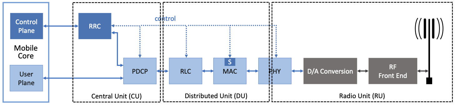
Radio Unit (RU). This sits at the cell site, on the tower or rooftop. It handles the analog-to-digital conversion, the RF frontend, and the lowest physical-layer (low-PHY) functions: Fast Fourier Transform (FFT) and its inverse (IFFT), cyclic prefix insertion and removal, and digital beamforming [7][9]. These are the functions that must run at the speed of the radio — microsecond timescales — and cannot tolerate any transport delay.
Distributed Unit (DU). This sits near the cell site — possibly at the base of the tower, possibly in a small edge facility within a few kilometers. It runs the high-PHY functions (channel coding and decoding, modulation and demodulation, HARQ processing), the MAC layer (the scheduler itself), and the Radio Link Control (RLC) layer (segmentation and reassembly) [7]. The DU operates at millisecond timescales — the TTI clock.
Central Unit (CU). This sits further back — in a regional data center, potentially serving tens or hundreds of cells. It runs the Radio Resource Control (RRC) layer (connection management, handover decisions, measurement configuration), the Packet Data Convergence Protocol (PDCP) layer (header compression, ciphering, reordering), and the new Service Data Adaptation Protocol (SDAP) layer (mapping QoS flows to data radio bearers) [7]. The CU operates at timescales of 10 to 100 milliseconds — slow enough to centralize, fast enough to adapt.
The interfaces between them are standardized: F1 connects CU to DU [7]. E1 connects the CU’s control-plane and user-plane halves (the CU itself can be further split into CU-CP and CU-UP) [7]. Open Fronthaul connects DU to RU [9].
The functional split: why 7-2x?
The split point between DU and RU is the critical design decision. 3GPP defined eight possible split options, numbered 1 through 8, with Option 8 being the lowest (raw I/Q samples shipped from the RU to a remote processor) and Option 1 being the highest (almost everything stays at the radio site) [7].
Option 8 is the legacy C-RAN approach: the RU is a “dumb” radio head shipping raw digitized samples over CPRI (Common Public Radio Interface) [13]. This gives maximum centralization — all processing is pooled — but the bandwidth is enormous. A single 100 MHz 5G NR carrier with 4 antenna ports generates roughly 157 Gbps of raw I/Q data [6]. Where does that number come from? CPRI digitizes each antenna’s analog signal at the Nyquist rate (2× the bandwidth = 200 Msps for 100 MHz), with each sample represented as a pair of 16-bit values (I and Q components) plus CPRI framing overhead (~25%). Per antenna: 200M × 32 bits × 1.25 overhead ≈ 8 Gbps. Across 4 antennas and accounting for additional control/synchronization overhead, the total reaches roughly 40 Gbps per carrier — and the 157 Gbps figure from Rost et al. [6] accounts for wider configurations (multiple carriers, higher-order MIMO). The point: fronthaul bandwidth scales linearly with both antennas and channel width. Massive MIMO with 64 antennas would require terabits per second of fronthaul. CPRI breaks.
Option 7-2x is the compromise that 5G and O-RAN adopted [9]. The RU performs the low-PHY processing — FFT/IFFT, beamforming — and ships frequency-domain symbols rather than raw time-domain samples. This reduces fronthaul bandwidth by roughly 10x compared to Option 8 while keeping the latency-critical HARQ processing at the DU [2]. The “x” in 7-2x refers to a specific variant within the Option 7 family where precoding (beamforming weight application) is performed at the RU, further reducing fronthaul load [9].
The fronthaul latency constraint
Why can’t the DU sit anywhere? Because of HARQ timing. Hybrid Automatic Repeat Request (HARQ) is the mechanism by which the receiver (either UE or gNB) acknowledges or requests retransmission of each transport block [11]. The timing is strict: after receiving data, the UE expects an ACK or NACK within a fixed number of slots. In 5G NR with 30 kHz subcarrier spacing (the most common mid-band configuration), the HARQ round-trip budget is approximately 4 milliseconds [11]. The DU must decode the uplink transport block, decide ACK or NACK, and get the response back to the RU for transmission — all within that window.
Subtracting processing time at both ends leaves roughly 250 microseconds for one-way fronthaul transport [1]. At the speed of light in fiber — approximately 200 meters per microsecond (5 microseconds per kilometer) — this limits DU placement to within about 20 kilometers of the RU. That is a hard physical constraint. You cannot put the DU in a distant data center; you need edge infrastructure within that radius.
This is a concrete instance of what the course framework calls decision placement [10]: the fastest decisions (HARQ, scheduling) must stay physically close to the radio because latency is dictated by physics. Slower decisions (RRC connection management, handover policy) can migrate further back to the CU, which can sit in a regional data center tens of milliseconds away. And the slowest decisions (network-wide optimization, ML model training) can sit even further back, in the cloud. The split is not arbitrary — it is forced by the timescale of each function.
Framework reading
Pause and notice what just happened. The design principle is disaggregation — the same principle we identified in Lecture 3 when we studied how the Internet evolved from monolithic IMPs to modular routers with separable forwarding and control planes. The gNB underwent the same trajectory: a monolithic box that was cracked open along the seams where timescale requirements diverge. Microsecond functions (RF, beamforming) stay at the RU. Millisecond functions (scheduling, HARQ) move to the DU. Tens-of-milliseconds functions (RRC, PDCP) move to the CU. The split points are not design preferences — they are forced by the physics of latency.
And disaggregation here is not an abstract principle. It has a concrete economic payoff: CU processing can be pooled across many cells in a centralized facility, achieving the statistical multiplexing gain that C-RAN promised. DU processing can be shared across a smaller cluster of nearby cells at an edge site. Only the RU remains per-cell. Capital cost drops. Utilization rises.
Part 2: O-RAN — Opening the Interfaces
Disaggregation split the base station into pieces. But who makes each piece? In the legacy model, the answer was: one vendor. You bought your CU, DU, and RU from Ericsson, or from Nokia, or from Samsung. The interfaces between them — even the standardized ones like F1 — were implemented with proprietary extensions. Mixing a Nokia DU with an Ericsson RU was theoretically possible, practically impossible. The vendor lock was the cellular equivalent of the pre-SDN router world: vertically integrated stacks where innovation required vendor cooperation and vendor timelines.
This is the Interface invariant, and it was closed.
The SDN parallel
If this sounds familiar, it should. In Lecture 4, we studied Software-Defined Networking. Before SDN, routers were vertically integrated: Cisco or Juniper shipped a box with the data plane (packet forwarding) and control plane (routing protocols) tightly coupled, running proprietary software on proprietary hardware. You could not inspect the forwarding table format, modify the routing algorithm, or replace the control plane without replacing the entire router.
OpenFlow changed that by defining a standard interface between the control plane and the data plane. Once the interface was open, the control plane could be software running on commodity servers, independently developed and deployed. Data-plane hardware could be commoditized. Innovation in control-plane algorithms — routing, traffic engineering, load balancing — exploded. The cost of building a network dropped by orders of magnitude. Arpit has mentioned buying a 6.4 Tbps switch for twelve thousand dollars — a device whose equivalent would have cost hundreds of thousands in the pre-SDN era.
O-RAN is the cellular SDN moment.
The O-RAN Alliance
The O-RAN Alliance formed in 2018 from the merger of the xRAN Forum and the C-RAN Alliance [9]. Its mission: define open interfaces for the disaggregated RAN so that operators can mix vendors, deploy third-party optimization software, and reduce their dependence on any single equipment provider [2].
O-RAN builds on top of 3GPP’s CU/DU/RU split [2]. It does not replace 3GPP standards — it extends them with additional open interfaces and a new control layer. The key additions are:
Open Fronthaul. O-RAN standardized the Option 7-2x split interface between DU and RU for multi-vendor interoperability [9]. A compliant RU from vendor A should work with a compliant DU from vendor B. In practice, interoperability testing remains expensive and imperfect — this is the integration tax — but the principle is established.
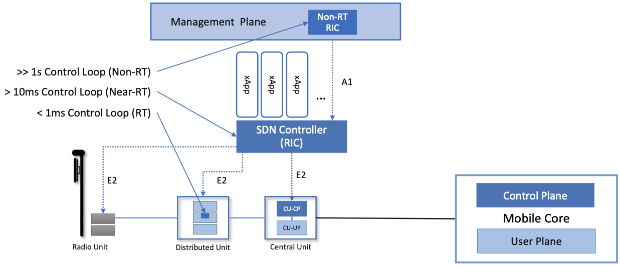
The E2 interface. This connects the RAN (CU and DU) to a new entity: the Near-Real-Time RAN Intelligent Controller (Near-RT RIC) [9]. E2 carries two kinds of traffic: telemetry flowing upward (E2 Service Model reports — per-UE channel quality, per-cell load, HARQ statistics) and control actions flowing downward (scheduling hints, handover commands, beamforming adjustments) [2]. The E2 Service Model (E2SM) defines what data can be reported and what actions can be taken — it is the API contract between the RIC and the RAN [9].
The A1 interface. This connects a Non-Real-Time RAN Intelligent Controller (Non-RT RIC) to the Near-RT RIC [9]. A1 carries declarative policy — not per-UE control actions, but strategic directives. For example: “prioritize the URLLC slice in cells 15-30 during the next hour” or “deploy this updated ML model for handover prediction.” A1 is the slow channel for strategic intent [2].
The O1 interface. This connects the Service Management and Orchestration (SMO) framework to all O-RAN network elements — CU, DU, RU, and the Near-RT RIC itself [9]. O1 handles configuration, performance management, and fault management. It is the operations interface.
The RAN Intelligent Controller
The RIC is the centerpiece of O-RAN’s contribution [2]. It introduces programmable intelligence into the RAN — the ability for operators and third parties to deploy optimization algorithms that observe RAN telemetry and inject control actions, without modifying the DU or RU firmware [3].
The RIC operates at two timescales:
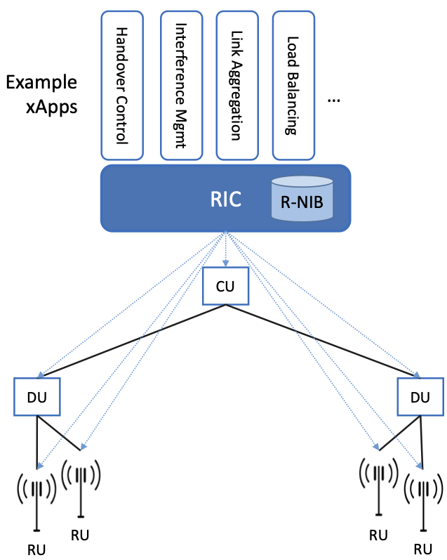
Near-RT RIC (10 milliseconds to 1 second loops). This runs applications called xApps — third-party software modules that implement specific RAN optimizations [3]. An xApp might optimize handover decisions by predicting UE mobility patterns from E2 telemetry. Another might manage inter-cell interference by coordinating beam directions across neighboring cells. A third might implement slice-aware scheduling — adjusting resource allocation across slices based on real-time SLA compliance [3]. Each xApp consumes E2 telemetry, runs its algorithm, and injects control actions back via E2. The 10 ms to 1 s timescale is fast enough to influence per-UE decisions but slow enough that the xApp does not need to run at the TTI clock speed of the DU scheduler [2].
Non-RT RIC (greater than 1 second loops). This runs applications called rApps — strategic optimization modules that operate on longer timescales [2]. An rApp might train an ML model on hours of historical E2 data, then push the trained model to a Near-RT RIC xApp via A1 [12]. Another rApp might analyze network-wide performance trends and generate policy updates. The Non-RT RIC is hosted inside the SMO framework and has a global view of the entire RAN deployment [9].
Three nested control loops
Step back and count the control loops that now exist in the system:
Loop 1: MAC scheduler at the DU (sub-millisecond to millisecond). This is the fastest loop. Every TTI — every millisecond or less, depending on the subcarrier spacing — the DU scheduler examines CQI (Channel Quality Indicator) reports from UEs, checks the QoS requirements of each flow, and allocates Physical Resource Blocks (PRBs) to UEs. This loop has always existed; it is the scheduling engine we have discussed since L8. It runs on specialized hardware or optimized software at the DU and cannot tolerate external interference at its timescale.
Loop 2: Near-RT RIC xApps (10 ms to 1 second). This loop observes aggregated telemetry from the DU — not raw per-TTI data, but windowed statistics (average throughput per UE over the last 100 ms, HARQ failure rates per cell, interference measurements) [3]. Based on this, xApps make medium-timescale decisions: adjust handover thresholds, shift resources between slices, update beamforming configurations. These decisions are injected back into the DU via E2, where they modify the parameters the MAC scheduler uses — but the xApp does not replace the scheduler. It tunes the scheduler [4].
Loop 3: Non-RT RIC rApps (greater than 1 second). This loop sees the broadest view and operates on the slowest timescale. rApps analyze trends across the entire network, train ML models, generate policies, and push them to the Near-RT RIC via A1 [2]. An rApp might detect that a cluster of cells consistently violates URLLC SLA during rush hour and push a policy that pre-allocates additional PRBs to the URLLC slice during those hours.
Each loop’s bandwidth is deliberately slower than the one below. This is the classic control-theoretic cascade: the fastest loop stabilizes the plant (radio channel), the middle loop optimizes the setpoints, and the slowest loop adapts the strategy. If a fast loop and a slow loop try to control the same variable at similar speeds, they oscillate — each one correcting the other’s corrections. The timescale separation prevents this.
This is closed-loop reasoning from Lecture 3, formalized as infrastructure. GSM had implicit control loops (power control, handover based on signal strength). LTE had explicit but narrow loops (eICIC for inter-cell interference). O-RAN made the loop hierarchy a first-class architectural element, with standardized interfaces at each boundary.
Framework reading
The Interface invariant is being opened — the same move as SDN opening the router’s control plane via OpenFlow. Before O-RAN, the RAN was a black box: the operator bought it, deployed it, and waited for the vendor to ship updates. After O-RAN, the operator can deploy third-party xApps that observe and influence the RAN’s behavior through standardized APIs.
The decision placement principle is explicit in the three-loop hierarchy. Fast decisions stay at the DU because latency is physical. Medium decisions move to the Near-RT RIC because they need a multi-cell view that no single DU has. Strategic decisions move to the Non-RT RIC because they need historical data and global scope that no Near-RT RIC has. The invariant rule: the speed of the decision determines its placement in the hierarchy.
But opening the interfaces creates a new problem: coordination among xApps. If xApp-A (a throughput optimizer) wants to hand over UE U to cell X for better channel conditions, and xApp-B (an energy optimizer) wants to keep UE U on cell Y so that cell X can go into low-power sleep mode, which one wins? This is the xApp conflict problem [4], and it is today what BGP policy oscillation was in the late 1990s — a distributed control problem whose pathologies emerge only at scale. In single-vendor pilots, where one vendor ships a coherent set of xApps, conflicts are rare. As the ecosystem grows and independent developers ship xApps with independent objectives, the conflict problem will sharpen.
Part 3: Network Slicing
We have disaggregated the base station and opened its interfaces. But there is a third pressure that 5G must address, and it comes from the demand side rather than the supply side.
The problem: contradictory requirements
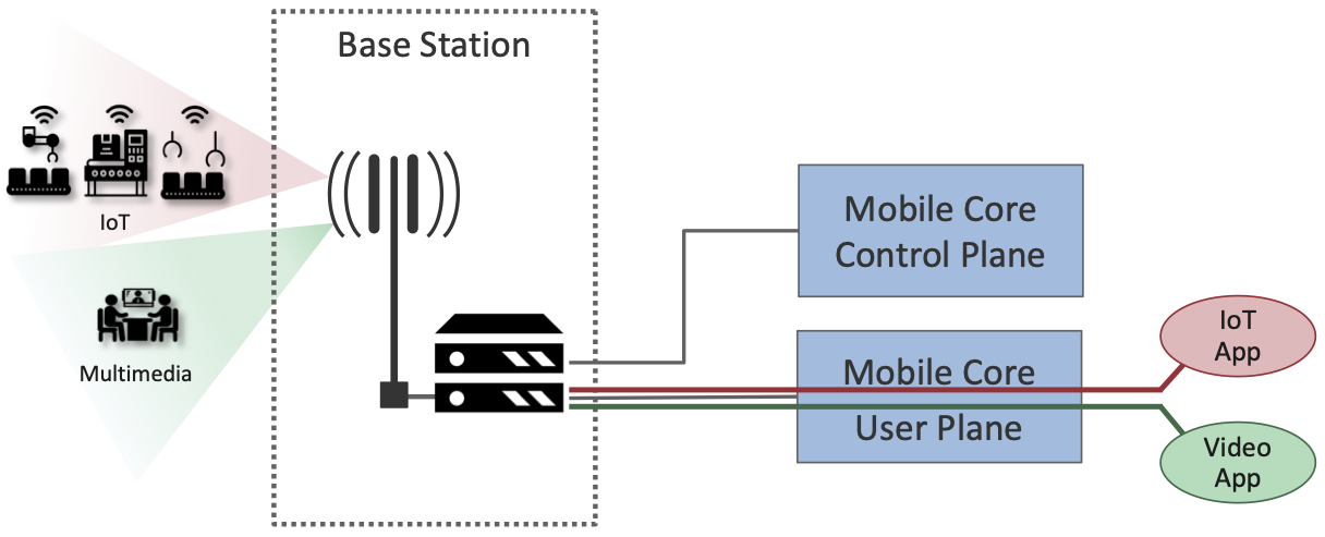
5G was designed to serve three fundamentally different service categories [14]:
Enhanced Mobile Broadband (eMBB). This is the successor to what LTE already does well: high-bandwidth data for smartphones, video streaming, and web browsing. The requirement is throughput — peak rates of 20 Gbps downlink, 10 Gbps uplink [14]. Latency is best-effort; reliability is standard. This is the service profile of a person streaming 4K video on a train.
Ultra-Reliable Low-Latency Communication (URLLC). This is new territory. The requirement is deterministic: 1 millisecond end-to-end latency and 99.999 percent reliability (five nines — no more than one failure in 100,000 transmissions) [14]. This is the service profile of a remote surgery system or an autonomous vehicle’s collision-avoidance link. Bandwidth is modest — perhaps a few hundred kilobits per second — but every packet must arrive on time, every time.
Massive Machine-Type Communication (mMTC). This is the Internet of Things at scale: up to one million devices per square kilometer [14]. Each device sends tiny packets — a few bytes of sensor data — infrequently, perhaps once every few minutes. Latency tolerance is generous (seconds). Reliability requirements are moderate. But the sheer number of devices is overwhelming: the signaling overhead of one million device registrations, connection setups, and keep-alives can swamp the control plane.
These three profiles have contradictory requirements. A scheduler optimized for eMBB maximizes throughput by giving resources to users with the best channel conditions — the opportunistic scheduling approach. But this is exactly wrong for URLLC, which needs guaranteed resources for a specific user at a specific time regardless of channel conditions. And mMTC needs the control plane to handle massive concurrent connections, which means lightweight signaling — the opposite of the rich per-UE state that eMBB and URLLC schedulers maintain.
You cannot build one scheduler that optimizes for all three simultaneously. The optimization objectives conflict.
The solution: network slicing
Network slicing is the answer: create logically isolated virtual networks — slices — on top of shared physical infrastructure [5]. Each slice gets its own set of Network Functions, its own scheduling policy, its own resource allocation, and its own Service Level Agreement (SLA). From the perspective of a tenant (an enterprise, a vertical industry, a service class), it looks like a dedicated network. From the perspective of the operator, it is one physical infrastructure serving multiple tenants [1].
A slice is identified by S-NSSAI (Single Network Slice Selection Assistance Information), a composite identifier with two parts [8]. The Slice/Service Type (SST) is a standardized 8-bit value: SST=1 for eMBB, SST=2 for URLLC, SST=3 for mMTC [8]. The Slice Differentiator (SD) is an optional 24-bit value that distinguishes among slices of the same type — for example, two different enterprise URLLC slices with different SLA parameters [8].
When a UE (User Equipment — a phone, sensor, or vehicle) registers with the network, it presents its desired S-NSSAI [8]. The registration flow passes through a chain of 5G core functions, each handling one concern:
- The NSSF (Network Slice Selection Function) reads the S-NSSAI and selects the correct slice — think of it as a load balancer that routes the attach request to the right virtual network [8].
- The AMF (Access and Mobility Management Function) handles registration, authentication, and mobility tracking for that slice — it is the 5G successor to LTE’s MME, but now per-slice rather than shared [8].
- The SMF (Session Management Function) sets up the data session — IP address allocation, QoS policy enforcement, tunnel establishment — analogous to a session controller [8].
- The UPF (User Plane Function) forwards the actual data packets between the RAN and the external network — analogous to a router in the data path. Crucially, UPF placement determines data-plane latency: a UPF at the network edge (near the DU) gives low latency for URLLC; a UPF in a central data center is cheaper but adds transport delay [8].
On the RAN side, the slice ID maps to scheduling priorities and resource pools at the DU [5].
Hard vs. soft isolation
The fundamental tension in network slicing is between isolation and multiplexing gain [5].
Hard isolation means dedicating physical resources to each slice. Slice A gets PRBs 1 through 50. Slice B gets PRBs 51 through 100. No sharing. The SLA is guaranteed — Slice A’s traffic cannot be affected by Slice B’s traffic because they operate on completely separate radio resources. But the cost is zero multiplexing gain. If Slice A is idle at 3 AM, its 50 PRBs sit empty. Nobody else can use them. The operator pays for capacity that goes unused.
Soft isolation means sharing resources with priority arbitration. All slices draw from the same pool of PRBs. A priority scheduler ensures that URLLC traffic gets first access, eMBB gets the remainder, and mMTC fills gaps. Multiplexing gain is high — idle capacity in one slice is immediately available to others. But SLA guarantees weaken under contention. If eMBB traffic surges and URLLC’s priority scheduler cannot preempt fast enough, URLLC packets miss their 1 ms deadline.
Real deployments blend both: a guaranteed minimum allocation (hard floor) plus best-effort oversubscription (soft ceiling). The URLLC slice might reserve 10 dedicated PRBs (guaranteed, always available) and have priority access to 20 additional shared PRBs (available unless contended). This hybrid approach trades some multiplexing gain for bounded-worst-case SLA compliance.
Framework reading
Network slicing is decision placement applied to resource partitioning. Where does the slice boundary live? How much isolation versus multiplexing? These are placement decisions on a continuum, and the answer depends on the service profile. URLLC pushes toward hard isolation because the cost of an SLA violation (a dropped surgery command, a missed collision warning) is catastrophic. eMBB tolerates soft isolation because a momentary throughput dip is annoying but not dangerous. mMTC tolerates even softer isolation because individual sensor readings can be delayed or retransmitted.
Slicing also applies disaggregation to the network itself — one physical infrastructure, N logical networks, each with independent NFs, state, and policy. And closed-loop reasoning enters at the orchestration layer: the Network Slice Management Function (NSMF) monitors per-slice SLA compliance and reallocates resources when drift is detected. If the URLLC slice’s 99.999% reliability drops to 99.99%, the NSMF can allocate additional dedicated PRBs or preempt eMBB traffic — a feedback loop at the orchestration timescale (seconds to minutes).
The unsolved problem is cross-domain orchestration. A slice is end-to-end: it spans the RAN (scheduling, PRB allocation), the transport network (fronthaul and backhaul capacity), and the core (NF instances, UPF placement). Orchestrating across all three domains — each with its own management stack, its own vendor, its own timescale — is where network slicing remains immature. And cross-operator slice federation (a URLLC slice that works while roaming between T-Mobile and Vodafone) is barely off the drawing board.
Part 4: The Grand Arc
The trajectory
Step back and look at the full arc that these five lectures have traced.
L5 gave us ALOHA — no state, no coordination, pure contention. Throughput ceiling: 18%. The system had no information about anyone else.
L6 gave us CSMA/CA — local state (carrier sense), distributed coordination (random backoff), the feedback loop completed with ACKs. The contention ceiling rose but remained structural. Bianchi proved it.
L7 showed WiFi fighting the ceiling with PHY improvements (modulation, MIMO, channel width) and MAC patches (aggregation, TXOP), all of which made the pipe wider but did not fix the coordination problem. Density finally broke the distributed model, and 802.11ax centralized the MAC with OFDMA and Trigger Frames.
L8 traced cellular’s parallel path: GSM’s monolithic TDMA scheduling, CDMA’s soft capacity, LTE’s OFDMA — always centralized, but progressively more flexible. WiFi and cellular converged on the same architecture: centralized OFDMA scheduling at millisecond timescales.
L9 — today — cracked open the centralized scheduler itself. 5G disaggregated the gNB into CU, DU, and RU along timescale boundaries [7]. O-RAN opened the interfaces and added programmable control loops at three timescales [2]. Network slicing virtualized the entire infrastructure to serve contradictory service requirements on shared hardware [5].
The pattern is the same one that the Internet followed: monolithic IMP (1969) to modular router (1980s) to software-defined network (2008). The cellular RAN followed: monolithic BTS (1991) to disaggregated gNB (2018) [7] to programmable O-RAN platform (2020) [9]. Disaggregation, then open interfaces, then programmable control. The sequence is not coincidental — it is forced by the same economic and technical pressures: vendor lock-in becomes intolerable, hardware utilization demands pooling, and service diversity demands programmability.
Three design principles across the arc
Disaggregation is the through-line. GSM’s monolith became UMTS’s bifurcated core, which became LTE’s flat EPC, which became 5G’s CU/DU/RU split plus Service-Based Architecture in the core, which became O-RAN’s separation of control logic from the data path, which became slicing’s per-tenant logical networks. Every generation separated what the previous generation had coupled. Every separation created a new interface. Every interface became a coordination point that had to be managed.
Closed-loop reasoning became explicit infrastructure only in 5G. GSM had implicit loops (power control at 800 Hz, handover based on signal strength measurements). LTE added eICIC (enhanced Inter-Cell Interference Coordination — neighboring eNodeBs negotiate which resource blocks to mute so cell-edge users suffer less cross-cell interference) and CoMP (Coordinated Multi-Point — multiple eNodeBs jointly transmit to or receive from a single UE, turning inter-cell interference into useful signal) at millisecond timescales. O-RAN formalized a three-loop hierarchy — MAC TTI at the DU, Near-RT RIC at 10 ms to 1 s, Non-RT RIC above 1 s — with each loop’s bandwidth calibrated to avoid oscillation with the loops above and below it [2][3].
Decision placement traced a continuum from “all decisions at the MSC” in GSM to “fast decisions at the DU, medium decisions at the Near-RT RIC, strategic decisions at the Non-RT RIC” in O-RAN. The invariant rule crystallized across the arc: fast decisions stay close to the radio because latency is physical; slow decisions migrate to centralized orchestrators because global view is needed.
The invariant evolution
Track how each invariant evolved across the five-lecture arc:
| Lecture | State | Coordination | Time | Interface |
|---|---|---|---|---|
| L5 (ALOHA) | None | None | Slot boundaries | None |
| L6 (CSMA/CA) | Local (carrier sense, backoff counter) | Distributed (random backoff) | Frame-time (~12 ms) | Minimal (busy/idle) |
| L7 (802.11ax) | AP-aggregated (per-client CQI, buffer) | Centralized (OFDMA scheduler) | Scheduling cycle (~1-5 ms) | OFDMA RU assignment |
| L8 (LTE) | BS-aggregated (CQI, QCI per UE) | Centralized (OFDMA scheduler) | TTI (1 ms) | Proprietary telco |
| L9 (5G/O-RAN) | Distributed across CU/DU/RU + RIC | Hierarchical (three nested loops) | Multi-timescale (us/ms/s) | Open (E2, A1, O1, Open Fronthaul) |
State went from absent to local to aggregated to distributed-across-layers. Coordination went from absent to distributed to centralized to hierarchical. Time went from coarse slot boundaries to millisecond TTIs to a multi-timescale cascade. Interface went from nonexistent to minimal to proprietary to open. Each transition was forced by a binding constraint shift — from no coordination (ALOHA) to distributed coordination limit (CSMA/CA ceiling) to density (WiFi centralizes) to service diversity (5G disaggregates and programs).
Cliffhanger
We have spent five lectures on the question “who transmits when?” From ALOHA to CSMA/CA to OFDMA to disaggregated programmable RAN, the story has been about medium access — the problem of coordinating transmissions on a shared wireless channel.
Now we shift. After the midterm, we move to the question: “what happens to the data once it enters the network?” The packets have been successfully transmitted. They are in the network. What now? How do routers handle congestion? What happens when a queue fills up — do you drop packets from the tail, or do you drop them proactively before the queue fills? How does a video stream adapt when the network is congested? How do you measure the network’s performance in the first place?
Queue management, multimedia applications, and network measurement. The next act begins.
Generative Exercise: Hospital Slice Design
You are the network architect for a hospital deploying a private 5G network. The hospital needs three slices on shared infrastructure:
Slice 1: Patient monitoring (mMTC profile). 2,000 sensors — heart rate monitors, IV drip sensors, room environment sensors — each sending 100-byte updates every 10 seconds. Latency tolerance: 5 seconds. Reliability: 99.9%. The challenge: massive device count, tiny packets, modest requirements per device, but the aggregate signaling load for 2,000 device registrations and keep-alives is significant.
Slice 2: Teleradiology (eMBB profile). Radiologists viewing and sharing medical images — CT scans, MRIs — that are 50 to 500 megabytes each. Latency tolerance: seconds. Reliability: 99.9%. Bandwidth requirement: sustained 100 Mbps per session, with bursts to 1 Gbps. The challenge: high sustained throughput without starving the other slices.
Slice 3: Remote surgery (URLLC profile). A surgical robot controlled by a surgeon in another building. Control commands: 200-byte packets at 1,000 per second. Video feedback: 50 Mbps 4K stereo stream. Latency requirement: 1 ms end-to-end. Reliability: 99.999%. The challenge: any packet loss or latency spike can cause the robot to make an incorrect movement.
Design questions:
For each slice, specify the S-NSSAI (SST and SD). Which standard SST values apply?
What isolation model would you use for each slice — hard, soft, or hybrid? Justify each choice in terms of the cost of SLA violation versus the cost of wasted capacity.
Where must the UPF be placed for the surgery slice? Work through the latency budget: 1 ms total, minus RAN processing time (~0.5 ms for encoding, scheduling, and transmission), minus core processing time (~0.1 ms). How much is left for transport? What does that imply about UPF placement?
The hospital wants to save money by using soft isolation between the monitoring and teleradiology slices, since neither has stringent latency requirements. Is this safe? What happens at 7 AM when 2,000 sensors reconnect after a nightly firmware update and 50 radiologists start their morning reads simultaneously?
The surgery slice is used 4 hours per day. Hard isolation reserves dedicated PRBs 24/7. What fraction of those PRBs is wasted? Can you design a hybrid scheme where the surgery slice has hard-reserved PRBs only during scheduled procedures and soft-priority access otherwise?
Think about this for three minutes, then discuss with your neighbor. We will work through the design together.
References
[1] L. Peterson and O. Sunay, Private 5G: A Systems Approach, Version 1.1, 2024. Available: https://5g.systemsapproach.org
[2] M. Polese, L. Bonati, S. D’Oro, S. Basagni, and T. Melodia, “Understanding O-RAN: Architecture, Interfaces, Algorithms, Security, and Research Challenges,” IEEE Communications Surveys & Tutorials, 2023.
[3] L. Bonati, S. D’Oro, M. Polese, S. Basagni, and T. Melodia, “Intelligence and Learning in O-RAN for Data-Driven NextG Cellular Networks,” IEEE Communications Magazine, 2021.
[4] S. D’Oro, L. Bonati, M. Polese, and T. Melodia, “OrchestRAN: Network Automation through Orchestrated Intelligence in the Open RAN,” IEEE INFOCOM, 2022.
[5] X. Foukas, G. Patounas, A. Elmokashfi, and M. K. Marina, “Network Slicing in 5G: Survey and Challenges,” IEEE Communications Magazine, vol. 55, no. 5, pp. 94-100, May 2017.
[6] P. Rost, C. J. Bernardos, et al., “Cloud Technologies for Flexible 5G Radio Access Networks,” IEEE Communications Magazine, vol. 52, no. 5, pp. 68-76, May 2014.
[7] 3GPP TS 38.300, “NR; NR and NG-RAN Overall Description; Stage 2,” Release 15, 2018.
[8] 3GPP TS 23.501, “System Architecture for the 5G System (5GS); Stage 2,” Release 15, 2018.
[9] O-RAN Alliance, “O-RAN Architecture Description,” v5.0, 2022.
[10] A. Gupta, A First-Principles Approach to Networked Systems, Ch. 4: Wireless Infrastructure, UC Santa Barbara, 2026.
[11] E. Dahlman, S. Parkvall, and J. Sköld, 5G NR: The Next Generation Wireless Access Technology, 2nd ed., Academic Press, 2020.
[12] S. Niknam, A. Roy, H. S. Dhillon, et al., “Intelligent O-RAN for Beyond 5G and 6G Wireless Networks,” IEEE Network, 2022.
[13] China Mobile Research Institute, “C-RAN: The Road Towards Green RAN,” White Paper, 2011.
[14] J. G. Andrews, S. Buzzi, et al., “What Will 5G Be?” IEEE JSAC, vol. 32, no. 6, pp. 1065-1082, June 2014.
© 2026 Arpit Gupta, UC Santa Barbara. All rights reserved. Contact the author for permissions.