Lecture 8: Hashing
\( \newcommand\bigO{\mathrm{O}} \)
1 Hashing
- The ability to address unique key values in an array whose size may be smaller than the set of possible key values.
- Generally, keys are unique values that identify some record of
information.
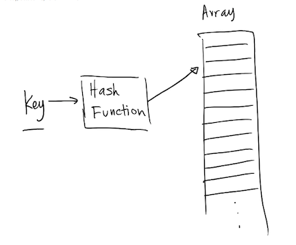
- In order to put data (value) in the appropriate place in the
collection, a hash function is required.
- The hash function outputs a position in the collection based on the key value
- Hash function outputs should be uniformly distributed
- Or else all data would try to be stored in the same index, and the table may degenerate to a linked list.
For example, if you have array of 100 elements, a simple hash function could be:
\[ key \mod 100 \in [0, 99] \]
- This is oftentimes a bad hash function if the table size is a power of 2
(why?), although the standard library uses this usually because it is
cheap to compute.
- Because it keeps only the lower bits of the integer and does not use the information in the higher bits.
- This is oftentimes a bad hash function if the table size is a power of 2
(why?), although the standard library uses this usually because it is
cheap to compute.
- Choosing a good hash function may be important, if you are using hash tables a lot. For example, using a faster but good hash function made some long-running (multiple hours-long) experiments \( 2 times \) faster in a research project I was working on earlier this year.
- In order to put data (value) in the appropriate place in the
collection, a hash function is required.
- Hashing is very efficient for searching for data in an array.
- Recall binary search: \( \bigO(\log n)\) search time (if elements are sorted).
- Linear search: \(\bigO(n)\) search time.
- Hash table search: \(\bigO(1)\) search time on average.
- Hash table searching provides instant access to an element in an array since the hash function computes the index where the data is stored.
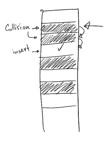
2 Collisions
- It's possible that two elements may be indexed to the same location.
- This is known as collisions
3 Open-addressing (confusingly a.k.a. closed hashing)
- Collisions are resolved by placing the item in another open spot in the array.
- One option for finding another open spot is to go through the array to find an
empty element. For example, if a record is hashed to position i and data
already exists in that index, then check the next available spot i+1, i+2,
etc.
- This is called linear probing
- What is a problem with this mechanism?
- Delayed Insertion – inserting an item in a crowded hash table
takes time since it must look for an empty spot.
- Elements are inserted farther away from their actual hashed index.
- Clustering – When different keys are hashed to the same index, there may be groups of data records grouped in the same place.
- Delayed Insertion – inserting an item in a crowded hash table
takes time since it must look for an empty spot.
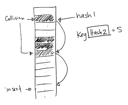
4 Double Hashing
Another option is to use a second hash function to resolve collisions.
- If a hash function index results in a collision, then use the 2nd hash function to determine how far to step in the array to look for an empty slot.
- Helps reduce the clustering effect.
- Problems
- If hash2 function is large, there is a possibility that we will go out of bounds. We resolve this by post-processing the output of hash2 to produce a value that is in-bounds. For example, we may use \( hash_2(x) \mod size \) to compute an index.
- Depending on the table size and hash2, it is possible that the indices won't be uniformly distributed.
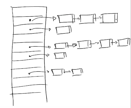
5 Chained Hashing
- The biggest problem to open-address hashing is
- If the table is full, no more elements can be added.
- Similar to a vector, it could expand the capacity "under-the-hood"
when needed, but…
- All elements will probably have to be rehashed (unless we cache the hashes).
- New capacity shouldn't be wasteful (too big) or too small.
- Chained hashing (chaining)
- If a collision occurs, then we store a series of data records in a list that the index in the hash table references.
- Linked Lists are a common collection to store collided data records.
std::unordered_mapuses this approach because it gives several nice guarantees:- All iterators/references to other elements are valid when an element is deleted/inserted.
- To guarantee this, the hash table can "re-wire" the chained linked lists.
- The main con of chained hashing is that now
findneeds to access another pointer to the linked list even on the first hit, so the data is less local.- There is a great (and long) talk at CppCon 2017 on evaluating different collision resolving schemes, with real-world performance data, if you want to see how sausage is made: https://www.youtube.com/watch?v=ncHmEUmJZf4
6 Growing and shrinking the table
Similar to a vector, we may want to grow the table when it is full. However,
if the table is too close to being full, then we will start having lots of
collisions and our table will perform badly.
Solution: grow the table when it is full enough to hurt performance, probably. We measure how full the table is using a value called load factor (denoted with \( \lambda \)):
\[ \lambda = \frac{\textrm{number of elements}}{\textrm{capacity}} \]
If the load factor grows beyond a threshold \( \lambda_1 \), then we resize the table and trigger re-hashing, similarly if the table was full.
On the other hand, after deleting a lot of elements, the table may be nearly empty, so we would want to reduce the wasted space. We can pick a second threshold \( \lambda_2 \), and when the load factor is less than this threshold then the table is too empty, so we shrink it and trigger re-hashing to save space.
The best values for the load factor thresholds would depend on our use case.
7 std::map vs std::unordered_map
- The underlying structure of an std::map is implemented with a balanced
tree structure.
- Useful if you care about the ordering of keys.
std::unordered_mapis used similarly to std::map, but thestd::unordered_mapis implemented with hash tables.- Notice the
std::unsorted_map's key / value pairs are not printed in sorted order by keys, butstd::map's keys are. - Hash Tables have a better amortized average case performance (O(1)), but data order is not guaranteed when traversing the structure with iterators.
- Notice the
| Operation | ~unordered_map~ | ~map~ | ||
| -- | Average | Worst-case | Average | Worst-case |
| Lookup | \(\bigO(1)\) | \(\bigO(n)\) | \(\bigO(\log n)\) | \(\bigO(\log n)\) |
| Delete | \(\bigO(1)\) | \(\bigO(n)\) | \(\bigO(\log n)\) | \(\bigO(\log n)\) |