CS190N Numb3rs -- Sniper Zero

The situation:

From the video, one is led to believe that Charlie is faced with a classification problem. From among the possible locations that a sniper could have used, which one is the most likely to have been the one this sniper chose given the observations Charlie makes of the aftermath of the crime. From our previous experience with Charlie's abilities, we know a little bit about "confidence," which, it turns out, is related to the statistical definition of the term "likelihood. If only Charlie had told us about how he was going to deal with uncertainty in his methodology.

Instead, he says that the problem is "fundamentally simple" and that one need only understand two physical "forces" -- vertical and horizontal velocity.

Let's get something straight. In this class, if you refer to "velocity" as a "force" your instructors are going to have, collectively, a series of brain hemorrhages. Help save them from this terrible fate and realize that velocity is not a force even when Charlie doesn't.

Returning to our hero, he seems to dream about attaching probabilities to locations, but he contends that from the observations of the "size of the wound," "angle of entry," and the "position of the body" it is possible to calcualte from where the shot has been fired. Notice that at this point, some discussion of uncertainty in the measurements or measurement error would turn this problem, potentially, into a statistics problem. No such luck. Charlie "knows."

So what calculations is Charlie doing in his head in order to determine the sniper's shooting location? From our own observations of Charlie, let's assume that the location of the body and the analysis of the wound give him, more or less, the direction from where the shot came. From there, as we can see in the show through Charlie's eyes, there are only a few feasible locations where a sniper might locate herself. To determine the most likely spot, then, one thing Charlie could do would be to compute the ballistic trajectory that fit all but one of his measurements (observations), solving the system for the missing measurement. For each feasible location he could then compare the measurement he solved for to the actual measurement and choose the one that is closest.

Or something.

If we believe that this is his methodology, from what he tells us and what we think he's looking at, it seems that the missing measurement he plans to use is the altitude of the sniper's location, given the direction, entry angle, and hortizontal range to the location. That is, all of the feasible locations that are in the direction of the shot are located at different altitudes. Thus Charlie's question seems to be

Given the horizontal range and the angle at impact, from what altitude was the shot fired?

Knowing the answer to this question, Charlie can compare the measured altitudes for his candidate locations and choose the one that is closest.

Certainly.

In attempting to figure out the answer to that question, one notices fairly quickly that Charlie must have some rather specific knowledge about bullets and the guns that fire them. In particular, even if someone measured out the horizontal and vertical distances for him (we only see him eyeball these values) he still need to know the horizontal and vertical velocities, say, at the point wheer the bullet was fired. We must presume that as a mathematician working at Cal Sci he is intimately acquainted with guns (although later in the show we find out that he's never fired one) and as a result he knows the muzzle velocity of the most likely offending rifle and also the horizontal distance from which the bullet was fired. We further postulate that he then solved some equations, in a matter of milliseconds, to determine the height from which the bullet was fired, and looked around to find the location that best matched his calculations. (The location he ended up choosing won with an impressive score of 87%; second place was 68%. As an activity for your own edification, write a paragraph or two describing what in the world those numbers might mean.)

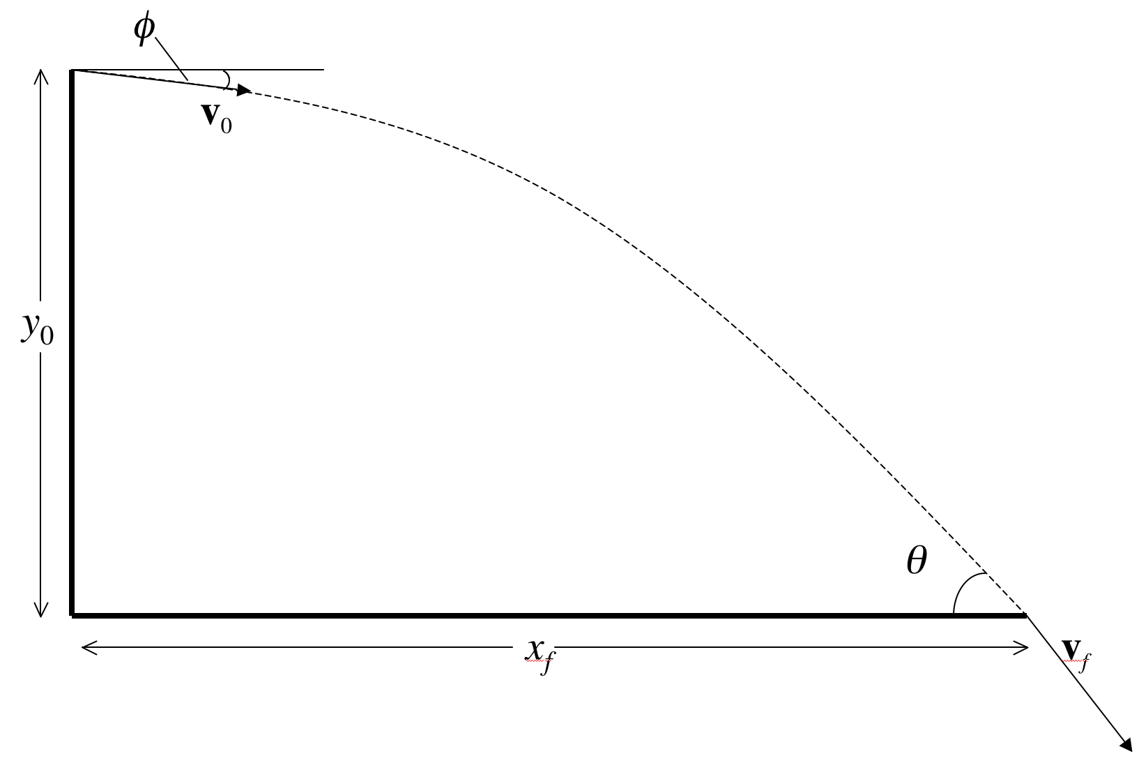
Thus we declare, from the luxurious back seat of the royal Fiat, that Charlie determined the horizontal distance x_f and that the rifle used delivered a muzzle velocity of v₀ f &frasl s to a 130-grain, 270-caliber Winchester deer-hunting bullet. (All of that info is actually germane here!)

It Would Be Cleaner with a Vacuum...

Now we can relate the angle &theta of impact with the initial angle &phi. Note that we can express

tan(&theta) = &minus ^v_y(t_f) ⁄_vx(tf) = ^{(gt_f + v₀sin(φ)}) ⁄_{v0 cos(φ)},  so
tan(&theta) = tan(&phi) + ^gx_f ⁄_{(v0 cos(φ))²} = tan(&phi) + ^gx_f ⁄_v0² sec²&phi = tan(&phi) + ^gx_f ⁄_v0² (1 + tan²(&phi)).

If &theta and x_f are known, as they are in our formulation of the problem, this gives us an quadratic in tan(&phi) that we can solve using the Quadratic Formula: this web page does the job nicely.

In case you are the old-fashioned type and you'd like to see how this goes by hand, recall that you need to solve the equation

tan(&phi) + ^gx_f ⁄_v0² (1 + tan²(&phi)) - tan(&theta) = 0

which should give you something like

^gx_f ⁄_v0²(tan²(&phi)) + tan(&phi) + (^gx_f ⁄_v0² - tan(&theta)) = 0

Now, does it look familiar? Obviously, you'll get two answers for values of tan(&phi) when you solve this equation. We'll take the positive one, since we have chosen v_y(t) to take on negative values; then we choose the principal value of arctan, since we surely want an angle in the first quadrant.

So knowing the muzzle velocity of the gun used (v₀) and the angle of entry (&theta) and the range x_f the acceleration due to gravity g for the planet you are on and that the planet has no atmosphere whatsoever, you can calculate the angle Charlie calls the "inclination of the gun" by solving the quadratic equation shown above. Do that in your head. We'll wait. Got it?

You are thus prepared to compute y₀ -- the height from which the bullet was fired. In particular, you already know that y(t_ƒ) = 0 at impact. Clearly, then,

y₀ = 0.5gt_f² + v₀ sin(φ) t_f

and since you know t_f in terms of the range x_f you know, without question or uncertainty, y₀ as Charlie does.

...but Real Life is a Drag

The simplest, but not the most realistic, model for drag force is that its magnitude is proportional to the speed (magnitude of the velocity) of the moving object. This makes the drag vector (negatively) propotional to the velocity vector; in symbols, F_d = &minus kv. While we're at it, let's divide the equation F = ma by the mass m of the bullet, so the acceleration from the drag is also proportional to the speed, with a new constant c = ^k ⁄_m. Our vector equation thus becomes

a_d   =   ^dv⁄_dt = −cv.

Now, for the moment, and in fact for many subsequent moments, we're just going to assume that we know the constant of proportionality from the physical properties of the bullet &mdash more on that as things develop. The following expression for the total acceleration a then obtains:

a   =   ^dv⁄_dt = −cv &minus gj,

where j is the unit vector in the y-direction. We can easily break this equation into x- and y-components:

dvx⁄dt = − cvx dvy⁄dt = −g − cvy

The first of these is the archetype variables-separable differential equation: Remember how grown-up you felt in Calc I when you could bang this one out? If you, like me, miss that more innocent, carefree time, this one's for you:

^dv_x⁄_vx = − c dt
ln(v_x) = &minus ct + D
v_x(t) = Ke^{&minus ct}   (where K = e^D)
v_x(0) = v₀ cos(φ),   so   v₀ cos(φ) = K   and

vx(t) = v0 cos(&phi) e&minus ct.

Ahh, it just makes you wanna head back to the dorm room and raid the 0.3-cubic-foot fridge, doesn't it? After the wave of nostalgia passes, let's do a teensy reality check. The x-velocity shows "exponential decay" from its original value, which I hope you'll agree is eminently sensible, given that, according to this model, its decay rate is proportional to its value. (Just like good ol' radioactive decay back in The Day!)

Despite its more frightening appearance, the v_y equation is not much harder: Make the substitution w = g + cv_y,  so that   ^dw ⁄_dt = c ^dv_x ⁄_dt. Then ¹ ⁄_c ^dw ⁄_dt = &minus w   and you get, as before, w = Ke^-ct   (different K, of course! We "freed" the K once we evaluated it above, so that we needn't come up with an ever-expanding sequence of names for constants.) Finally, substituting back in gives
v_y(t) = &minus ^g ⁄_c + Le^-ct   (L = ^K ⁄_c). Now,
v_y(0) = −v₀ sin(φ),   so   −v₀ sin(φ) = &minus ^g ⁄_c + L   and

vy(t) = &minus g ⁄c + (g ⁄c &minus v0 sin(&phi))e&minus ct.

Reality-check time again! (I can't overstate the importance of this ingredient to your problem-solving practices. You will make sign errors and silly arithmetic mistakes in your calculations. Making sure that your calculations jibe, at least on the surface, with reality as you go along will allow you to catch more of these mistakes before you have them engineered into your solution and will save you heartache in the long run that is equivalent many times over to the amount of time you spend on these simple checks. Word. I myself used this method to catch, and I'm perfectly serious here, over 26,000 of my own errors in the course of trying to solve the problem at hand.) What's going on here? Well, according to this model, the y-velocity approaches &minus ^g ⁄_c, the so-called terminal velocity, as t &rarr ∞. This should make us happy, because at some point, the acceleration of drag should balance with gravity; furthermore, the speed at which that occurs should be inversely related with the constant (more drag &rArr slower terminal velocity). By looking at the sign of the stuff in parentheses, we can even see that it speeds up to terminal velocity when v₀ sin(φ) < ^g ⁄_c and it slows down to terminal velocity when v₀ sin(φ) > ^g ⁄_c. Lovely!!

We now proceed with caution. First we'll find x, thence to determine the time t_f at impact; this will allow us to write down, much as before, an expression relating &theta and &phi, and we will finally be able to plug all that info into the gizmo we just found for v_y, find y(t), and declare victory. Happily, we can just integrate to solve the remaining differential equations. So:

x(t) = ^−v₀ ⁄_c cos(&phi) e^{&minus ct} + K   (Remember our convention about K!). Set x(0) = 0 to find
x(t) = ^−v₀ ⁄_c cos(&phi) e^{&minus ct} + ^v₀ ⁄_c cos(&phi),   or

x(t) = v0 ⁄c cos(&phi) (1 &minus e&minus ct). Right, then! As we are treating xf as a known constant, just set xf = x(tf) = v0 ⁄c cos(&phi) (1 &minus e&minus ctf). Rearranging then gives e&minus ctf = 1 &minus cxf ⁄v0 sec(&phi) (I record this here, because it will be convenient to sub it in this form a few steps down!) tf = &minus 1 ⁄c &sdot log(1 &minus cxf ⁄v0 sec(&phi)). Discussion Question for my minions who have taken to heart the above advice about reality checks: What if the thing inside the logarithm is negative? What then?? Huh??? I mean, we can't help it if  cxf ⁄v0 sec(&phi) just happens to be bigger than 1, can we? Explain in the context of reality. Next, we write an expression for tan(&theta), using all the hard work we've done so far: tan(&theta) = &minus vy(tf) ⁄vx(tf) = &minus (&minus g ⁄c + (g ⁄c &minus v0 sin(&phi))e&minus ctf) ⁄(v0 cos(&phi) e&minus ctf). A little algebra, which is frankly best done in the privacy of one's home, involving that e&minus ctf term I earmarked a few lines back gives the following simplified equation:   gxf ⁄v0 sec(&phi) + v0 sin(&phi) &minus cxf tan(&phi) tan(&theta) =    v0 cos(&phi) &minus cxf Before we get into how to solve this monster, let's Get Our Reality Check On one more time. What I'm looking for this time is some evidence of a connection between tan(&theta) and tan(&phi) &mdash after all, &theta is just an "adjustment" of &phi due to the various forces acting on the bullet &mdash and as a practical matter we don't expect the two angles to be all that different. First pass is to notice that if we set xf = 0, the expression reduces to v0 sin(&phi) ⁄v0 cos(&phi) = tan(&phi). Good: if the travel distance is 0, the angle darn well better not have changed! But we can do it one better: If you squint at the last two terms in the numerator, and you're a little weird like me, you might notice that they resemble the denominator. In fact, tan(&phi)(v0 cos(&phi) &minus cxf) = v0 sin(&phi) &minus cxf, so if we break up the fraction into two separate fraction, with the first term of numerator in the first fraction and the last two in the other, we get tan(&theta) = gxf sec(&phi) ⁄v0(v0 cos(&phi) &minus xf)   +   tan(&phi)(v0 cos(&phi) &minus cxf) ⁄(v0 cos(&phi) &minus cxf)   =   gxf sec(&phi) ⁄(v02 cos(&phi) &minus cv0xf)   +   tan(&phi), which displays tan(&theta) as equal to tan(&phi) with an "adjustment" term. (On top of all that, we see that the adjustment term is pretty small, because the v02 term in the denominator of the first term clobbers everything else!) Now to solving that equation. I'm not saying that someone cleverer than myself couldn't manipulate that equation and whip it into a nice quadratic in a trig function of φ or some other equation we have some hope of solving analytically; I will tell you, however, that I spent more time than I wish I did trying and not succeeding. No matter, however: We in the pedagogical stratosphere make lemonade out of lemons like these by using them as an excuse to Broaden Your Horizons. And no one is the worse for wear. No one, dear student, but you. A Small Treasury of Numerical Equation-Solving Methods, Both Stupid and Clever Suppose you're faced with an equation &mdash like the one above, for example &mdash and you want to find an approximate solution to within some given acceptable error. First off, let's suppose that we've solved for 0 and have the equation in the form ƒ (x) = 0; a solution to this equation is thus a zero, or root, of ƒ. We also need to assume that for any given x-value, we can calculate ƒ (x) to at least enough precision to allow us to find the root we're after. The Bad: Hunt-and-Peck... I guess that about the simplest thing you could do is to break up some interval into chunks of that size and evaluate the function at endpoints of each chunk, looking for an output value close to 0, and continuing to expanding the interval if the interval you chose didn't produce one. If you're lucky, then (a) you will find such an output and (b) it will be close to an actual solution. I don't recommend this method. The Better: Bisection... A substantially more clever method is that of bisection. Like most serious root-finding approaches, this method assumes that ƒ has some "nice" property; in this case, it's the mild condition that ƒ be continuous on some interval of interest. Here's how it goes: Find two x-values in your interval, say a and b, by any method you like, such that ƒ (a) and ƒ (b) have opposite signs. (If you can't find such an a and b, you might start to entertain serious doubts that your function has a zero at all!) The Intermediate Value Theorem, which sounds a lot scarier than it is, tells us that ƒ (x) has to be 0 somewhere on the interval (a,b). Now, evaluate the value of ƒ at the midpoint of (a,b), that is, ƒ (a+b ⁄2). This number is either 0, in which case we declare victory, or it has a different sign from one of the numbers ƒ (a) or ƒ (b), in which case there is a root between the midpoint and the appropriate choice of a or b by the reasoning above. Now, repeat the process with your new interval, which is half the size of the original. Keep repeating until you have it narrowed down to a tight enough tolerance. Example: Let's show how to use bisection to find a good approximation for √2. First, we should identify a function for which √2 is a root. Anyone? Yes, smarty-pants, the function ƒ (x) = x &minus √2 is certainly a function for which √2 is a root. The problem with that function is that you need to know the value of √2 in order to evaluate the function! Any better suggestions? Ah, yes, the world-famous function ƒ (x) = x2 &minus 2 will do nicely: We can surely evaluate this function to whatever precision we need, given a precise x-value, at least in principle. Let's start with a = 1 and b = 2; these are valid choices, since ƒ (1) = 1 &minus 2 = −1 and ƒ (2) = 4 &minus 2 = 2, and the numbers −1 and 2 notoriously have opposite signs. The midpoint of the interval (1 , 2) is 1.5, of course, and ƒ (1.5) = 2.25 &minus 2 = .25. Since .25 is opposite in sign to −1, we choose the interval (1 , 1.5) as the next one in the iterative process. The midpoint here is 1.25; ƒ (1.25) = −.4375; the next interval is thus (1.25 , 1.5), etc. Exercise: (i) Carry out two more full iterations of the above process.   (ii) How many iterations would this method require to find √2 accurate to six decimal places? Twenty decimal places? Is it Good? Darn Tootin': Newton's Method Provided that your function ƒ is not just continuous but differentiable on some interval of interest, we can use a much more efficient method. (Discussion Question: Think of a function that is continuous but not differentiable.) Newton's method is an itereative scheme that works as follows: Start with an initial guess x0 for your solution. Using the tangent line at (x0, ƒ (x0)) as an approximation for ƒ (x), find the x-value x1 where this line crosses the x-axis; this x1 will serve as the next guess. We can write down a simple expression for how to find x1 in terms of x0: The slope of this line is ƒ ′(x0), and the change in y along this line from x = x0 to x = x1 is 0 &minus ƒ (x0) = &minus ƒ (x0), so we end up with the equation ƒ ′(x0) = mtan = Δy ⁄Δx = −ƒ (x0) ⁄x1−x0. Multiply by (x1−x0), divide by ƒ ′(x0), add x0, put your left foot in, shake it all about, and you get x1 = x0  &minus   ƒ (x0) ⁄ƒ ′(x0). Now the iterative procedure falls into our lap like ripe fruit from the tree: Given xi at any stage in the process, xi+1 = xi  &minus   ƒ (xi) ⁄ƒ ′(xi) Is Newton's method infallible? No. Lots of things can go wrong. For one thing, if some ƒ ′(xi) = 0, we're in deep trouble. That said, it's not too likely in practice, since we tend to use this method for messy fucntions, ones for which the zeros of the derivative would be hard to find even if you were looking for them. Another thing that can go wrong is that ƒ ′(xi) might be so close to 0 that the ƒ (xi) ⁄ƒ ′(xi) term gets huge and knocks you miles away from the zero you were interested in finding. One of two things might happen from there: either you return, maybe rather slowly, to the zero of interest, or you've been thrown close enough to a different zero that Newton finds that one instead. A related problem is that there might be two points such that the algorithm just oscillates between the two; again, this isn't too likely and relies on extremely bad luck in choice of starting value. When Newton doesn't encounter this difficulty, which is most of the time, its rate of convergence is very rapid: Provided ƒ doesn't have a horizontal tangent line at our zero of interest, once you get sufficiently close to the zero, each iteration's error is about equal to a constant times the square of the previous one. That sounds better than it is, probably: Essentially, every iteration gives you roughly double the number of decimal places of accuracy as the last, after a point. Typically, Newton's method terminates when two successive xi agree to the prescribed accuracy. As a check, one can add and subtract the desired tolerance from one's final solution to make sure that the interval encloses a zero. Problem Write yourself a li'l ol' Newton's Method solver. With a starting value x0 = 1, find √2 accurate to six decimal places and to twenty decimal places as in the above exercise with the bisection method. Keep track of the number of iterations each requires and compare with the number you worked out for bisection. Here's the tricky part... Now that your Newton solver has all the bugs worked out of it, you can simply whack the above nasty equation with it and work out &phi to any desired level of accuracy. (Question for meditation: What would be a logical &phi0-value to use in this problem?) Despite its tempting appearance as the path of least resistance to getting our hands on a function, I will urge you not to go bolting for   gxf ⁄v0 sec(&phi) + v0 sin(&phi) &minus cxf tan(&phi) ƒ(&phi)   =     &minus   tan(&theta)   v0 cos(&phi) &minus cxf as the function to use, even though it is certainly correct to do so. Why? Well, remember that we're going to have to take a derivative; if you're like me, and I know I am, you'd just as soon avoid the Quotient Rule, especially if you can do so cheaply. The standard Newton's Method trick is to multiply both sides of your equation ƒ(x) = 0 by the common denominator. If we do that here, we get a new function that's still supposed to equal 0 but is much easier, in my humble view, to handle. (I hope you don't mind if I call it ƒ again.) ƒ(&phi) = gxf ⁄v0 sec(&phi) + v0 sin(&phi) &minus cxf tan(&phi) &minus (v0 cos(&phi) &minus cxf) tan(&theta). The aforementioned differentiation really isn't that bad: Remember, the only true variable in sight is &phi, so there are no products or quotients to handle. It's just ƒ ′(&phi) = gxf ⁄v0 sec(&phi) tan(&phi) + v0 cos(&phi) &minus cxf sec2(&phi) + v0 tan(&theta) sin(&phi). Now, are we done? Almost. Remember, we still need to find y0. Recall that way back in the Mesozoic, we derived the expression vy(t) = &minus g ⁄c + (g ⁄c &minus v0 sin(&phi))e&minus ct Integrating this with respect to t is pretty dang easy; it's just a constant and a constant times an exponential. y(t) = &minus gt ⁄c + (v0 sin(&phi) ⁄c   &minus   g ⁄c2) e&minus ct   +   K This formula, with all the known constants thrown in, will depend, through the constant of integration K, on the still unknown y0. Don't think for a second that I would deny you the pleasure of finding K, solving for y0 using the equation y(tf) = 0, and thus claiming your FBI Junior Detective Merit Badge for Outstanding Work in Linear Drag. Squaring With Reality At this point in the adventure, we surely feel edified but wary: Even as we bask in the well-deserved glow of a Job Well Done, those words "not the most realistic," used in reference to the previous drag model, haunt us. As it turns out, for macroscopic objects moving at more than a snail's pace, drag is not linear but fairly near to quadratic. (I have a physicist friend who tried to explain this stuff to me, but it didn't really take. I gather that, at very low velocities, the air behaves as though there are "layers" or lamina, one of which is sticking to the moving object. The successive layers are "sheared" apart, and that shear force ends up being, for reasons I don't understand, proportional to the object's speed. On the other hand, if the speed is high enough that the object is actually compressing the air in front of it, generating turbulence rather than just gliding along with the lamina, then the dominant force is the one opposing this compression &mdash which is proportional to the square of the speed, again for reasons that are obscure to me.) So, yes, that's right, let's take yet a third pass at this problem, this time with the much more realistic assumption that drag is proportional to the square of the speed of our bullet. This may at first blush seem as though it will be a trivial generalization of the last version of the problem, and as a vector equation it even looks kind of pretty: dv⁄dt = −c |v| v That first blush is replaced by a full-blown blanch, however, as it begins to dawn on us what we need to do in order to write down the equations in terms of x- and y-components. If we write dv⁄dt = c √(vx2+vy2) v, we see that dvx⁄dt = − c √(vx2+vy2) vx dvy⁄dt = −g − c √(vx2+vy2) vy The real upshot here is that, since the x-component of the acceleration of drag depends on the y-velocity, and vice versa, we can no longer separate the two differential equations and solve them separately from one another. Even I gave up trying to solve that mess analytically before too long! Once again, let's treat the constant of proportionality c as though it is known. In order to proceed, we're going to need to use some ideas from numerical integration, which we may or may not have seen before. Numerical Integration: Making it All Add Up Solving differential equations is, of course, intimately bound up with the concept of integration. Recall that the integral of a function over an interval is naïvely defined as the limit of sums of areas of rectangles, called Riemann sums, as pictured here. The function of interest, of course, is graphed in red, and the interval is [0, 2]. The theory says that you chop your interval up into sub-intervals, choose an x-value within each sub-interval (most typically the left endpoint, the right endpoint, or, as pictured above, the midpoint), to evaluate the function and thus determine the height of that sub-interval's rectangle; as you do this over ever-finer subdivisions of the interval, the sums of the areas of the rectangles approaches a limit, provided of course that the function is not too nasty, and this limit is the integral. Of course, the Fundamental Theorem of Calculus tells us that we can integrate by antidifferentiating, and we have spent most of the rest of our lives, including this course up to this point, whacking integration problems with that particular sledgehammer. However, like many perfectly well-meaning sledgehammers, this particular one is not an all-purpose tool. This reflects a cruel irony: The fact is that we can, at least in principle, differentiate just about any expression thrown together any way at all using the four basic operations of arithmetic, exponents, roots, logarithms, and trigonometric functions. However, it's a rather delicate matter, and often impossible, to find an explicit antiderivative of such an expression or to find an explicit solution for a differential equation built up in this way. On the other hand, most of the interesting and important applications involve, not differentiation, but integration and the solution of differential equations. Fortunately, these problems lend themselves particularly well to numerical methods. What I'd like to do is to give a brief synopsis of a few different numerical methods for solving differential equations and their more familiar counterparts back in Integration Land. For now, I'd like to assume that we are trying to solve a differential equation of the form x′(t) = ƒ(t,x), x(t0) = x0, where ƒ is a function that we know how to evaluate everywhere over a region of t-and x-values and x0 is a given constant "starting value." Under suitable hypotheses, there is a function x(t) satisfying the above differential equation, and our goal is to approximate this function; in particular, we may want to have an estimate for x(b) for some later t-value of interest, or we may want to know how "long" it takes for x to reach a certain value, etc. Notice that if ƒ happens to be a function of t alone, then the problem is really one of finding an approximation to the integral of ƒ over some interval. Euler's Method: Nice 'n' Simple This iterative method is easy to understand and straightforward to implement. Choose an increment h for your t-values, so that we will approximate values for x(t0+h), x(t0+2h), ... , until we reach some stopping criterion appropriate to the problem at hand. Recall the tangent-line approximation x(t0+h) &asymp x0 + hx′(t0) = hf(t0,x0). Now, write t1 = t0+h, x1 = x0 + hf(t0, x0) &asymp x(t1), and this begins the following iterative process: Given ti and xi, define ti+1 = ti+h, xi+1 = xi + hf(ti, xi). Euler's method corresponds to the left-endpoint approximation to an integral, with rectangle width h. To understand the connection, let's suppose that x&prime is a function of t alone, say ƒ(t), and let's write the antiderivative x(t) as ƒ(t), just to avoid confusion! With one rectangle of width h, the left-hand approximation is for the integral from t0 to t0+h of ƒ(t), and the calculation is just width &sdot height, or hƒ(t0). On the other hand, by the Fundamental Theorem, the integral in question is ƒ(t0+h) − ƒ(t0), and as we saw above, Euler's Method calls this quantity x(t0+h) &minus x(t0) = x1 &minus x0 and approximates it as (x0+hx′(t0)) &minus x0 = hx′(t0) = hƒ(t0). So the calculations agree for one interval, and for more intervals both methods add the contributions from the individual intervals, so they agree for any number of intervals. Conceptually, I think of the methods as agreeing because they both make the estimation based only on the beginning value on each interval and the interval width h. Example: Let's use Euler to give a numerical solution to the differential equation x′(t) = ƒ(x, t) = 2x ⁄t, x(1) = 2, using step size h = 0.1. Then x0 = 1 and ƒ(2, 1) = 4 ⁄1 = 4, so x1 = 2 + 0.1 &sdot 4 = 2.4. Next, t1 = 1.1, ƒ(1.1, 2.4) = 4.8 ⁄1.1 &asymp 4.364, so x2 &asymp 2.4 + 0.1 &sdot 4.364 = 2.8364. Exercise: Write a routine for doing Euler's method and carry it out for this example to find an approximate value for x(2). To check the accuacy of the solution so obtained, solve the above differential equation analytically (Answer: x = 2t2) to find the exact value of x(2). Back to the Problem: What Would Euler Do?   Enlightened as we now feel, how do we go about using Euler to help us find y0? Remember, that was the goal of this narrative in the first place. To that end, we make a couple of observations. The first is that the setup outlined above also applies to vector variables &mdash in this case, v = (vx, vy). The differential equation is now of the form v′(t) = ƒ(t, v); to be specific for our case, v′(t) = (− c √(vx2+vy2) vx, −g − c √(vx2+vy2) vy). So given &phi and initial speed v0, we can write down the initial velocity v0 = v(0) = (v0 cos(&phi), v0 sin(&phi)). Now, choose a value for h, and the iterative process looks like vi+1 = vi + hv′(ti). Furthermore, check this out: As you go along incrementing t, you can also update x and y as you're going along. Here's why: Since x′(t) = vx, you can use that selfsame Euler's Method on that differential equation, using x0 = 0, and write xi+1 = xi + h(vx)i, where (vx)i means just what you think it does, the value for vx that the Euler process calculates at step i. Same deal for y. And when do we stop? When xi gets to xf, of course! "Now, just a cotton-pickin' minute," you say, "we don't know &phi. You've said so yourself a hundred times." True enough, which brings me to my second remark. For the purposes of this and all other numerical approaches, let's just set y(0) = 0. Then the "final" y-value we produce will be a negative number, namely the opposite of the starting height. With this convention in place, note that once you've specified h and the stopping criterion on x, &phi is the only variable in determining the final values of x (which will be essentially equal to xf), y, vx, and vy. We can determine whether our choice of &phi is correct by comparing the final value of −vy ⁄vx and seeing whether it is equal to tan &theta. In symbols, if we call &weierp the big mysterious function that takes the value &phi, runs the Euler process until x &ge xf, and returns the final value of −vy⁄vx, this gives us an equation to solve, namely &weierp(&phi) &minus tan &theta = 0. This is a beautiful example of a non-analytic function that we can evaluate at any value we want, albeit at some computational expense. Have we met any numerical methods that would allow us to solve an equation like this one? I posit that, at least in principle, &weierp is a continuous function of &phi. I hope that makes intuitive sense; all it's saying is that if you change &phi by a small amount, &weierp(&phi) will also change by a small amount. At least, it's as continuous as it needs to be with respect to the issues of numerical precision that are foisted upon us by this imperfect world in which we live. Therefore, we might wonder whether or not the bisection method would work. I claim that it, in fact, would! Remember that we have a reasonable "starting guess" for &phi, namely the known angle &theta itself. Furthermore, if we use &theta for &phi, I think it's manifest that the angle you get at the end will be too large, so the left-hand side &weierp(&phi) &minus tan &theta will end up positive. (In fact, the first thing I would do after I wrote out the Euler's-method algorithm for this &weierp(&phi) would be to check that its calculated &weierp(&theta) > tan &theta.) So run the algorithm with successively smaller values of &phi until you get a negative value for &weierp(&phi) &minus tan &theta, and you're off to the races with the bisection algorithm! As mentioned above, after you do all that, the final value of y you get when you run the algorithm with the correct value of &phi will be the negative of the height above the entry wound that the bullet left the rifle. (Discussion Question: The conscientious, or at least conscious, reader may recall that Newton's Method was touted as vastly superior to bisection. Why do we not use Newton rather than bisection to solve that final equation?) Tempting as it is to declare victory and move on to other matters, we will not. The main issue is one of accuracy: Even for relatively small choices of step size h, the simplicity of the method makes it pretty darn inaccurate. If you think about the left-endpoint approximation for integrals, you'll begin to see why. Just look at all that area we missed! How much? Well, each of those little wedges is roughly the shape of a triangle. The width of the triangle is our stepsize h, and the height is roughly h times the slope of the graph (since m = &Deltay ⁄&Deltax, &Deltay = m&Deltax, and &Deltax = h). So the area of each triangle-like wedge looks something like 1 ⁄2 h2y&prime. Over an interval [a, b], there are b−a ⁄h such wedges, so the best really feel good about saying is that the error is no worse than 1 ⁄2 h(b−a)M, where M is some max value for the absolute value of y&prime on the interval. This is pretty bad! For example, suppose that you want to find the value, within 10−6, of the integral of a function from 0 to 5, and you know the derivative is never any larger than 10 or smaller than −10. Then you need h(5-0)⋅10 = 10−6, so h = 2ċ10−8. That means 25,000,000 sub-interval calculations to do. If you really wanted to ratchet down on it and get 12-place accuracy on your answer &mdash well, you'd better start now. And for Euler's method, the situation is even worse! The reason for this is that, in the left-hand endpoint method, at least we knew the exact (in principle) value of ƒ(ti) at each step, so the only error introduced is from what the function does along the subinterval. In the case of Euler's method, you use x(t0) to get an approximation x1 for x(t1), but then you have to use the approximated value x1 in your calculation for x2. If we somehow knew x(t1), the situation would only be as bad as left-hand endpoint integral approximations, but the error is now compounded by the fact that you approximated the point you needed to use in order to make your approximation! For these reasons, Euler's method is rarely used for serious problems. Heun's Method: It's A "Trapezeuler" Thing I hope that you recall the trapezoidal method for integration; it's a cheap and easy way to improve the accuracy of the left-hand endpoint method. The geometric motivation behind this method is pretty clear: instead of approximating the area over each sub-interval by a flat-topped rectangle, let's connect the dots along the graph, so that our strip of area now has a slanty top. Here's a picture: The ith strip in the approximated area is thus a trapezoid, the area of which is, as we may(!!) recall, base times average height, or h &sdot (ƒ(xi) + ƒ(x i+1))⁄2 . Thus the trapezoidal method doesn't require us to evaluate the function at any more points that Euler's does, but it does take into account the way the function changes over each sub-interval. The way it does this is with a simple linear approximation, not rocket science by any means but certainly better than nothing. And the trapezoidal method is more effective, in the sense that now the error is proportional to h2, rather than just h, so that decreasing h by a factor of 10 improves your accuracy by a factor of 100 or so. The diff-eq version of the trapezoidal method goes by the name of Heun's method or, catchily, the improved Euler method. So how would this method work? Suppose we're given, as usual, the information x′(t) = ƒ(t,x), x(t0) = x0, and suppose that we have decided on a step size h. Then, in the spirit of trapezoidialism, we'd like to define x1 to be x0 + h &sdot (ƒ(t0, x0) + ƒ(t1, x1))⁄2 . Of course, there's a small catch, namely that this would require us to know x1 ahead of time in order to calculate x1, so it's not quite possible to execute the step we want to. We thus resort to the following clever trick. Recall that Euler's method gave us the approximation x(t1) &asymp x0 + hf(t0, x0) &mdash let's call this value x1&lowast. Of course, the point is to do better than Euler's method, so we won't be using x1&lowast as our x1. Now here's the clever part: If x1&lowast is a fair approximation for x(t1), then ƒ(t1, x1&lowast) is a fair approximation for ƒ(t1, x(t1)) &mdash not perfect, but it's a safe bet that it's better than ƒ(t0, x0). Thus it will be a substantial improvement on Euler to use x1 = x0 + h &sdot (ƒ(t0, x0) + ƒ(t1, x1&lowast))⁄2 . This leads us easily to the iterative procedure xi+1&lowast = xi + hf(ti, xi) xi+1 = xi + h &sdot (ƒ(ti, xi) + ƒ(ti+1, xi+1&lowast))⁄2 . Heun's method is the of a class of so-called predictor-corrector algorithms &mdash so called because it first makes a prediction xi+1&lowast for xi+1, then corrects the prediction by an adjustment that uses the prediction itself. Example: Let's take another shot at the differential equation x′(t) = ƒ(x, t) = 2x ⁄t, x(1) = 2, step size h = 0.1. As before x0 = 1 and ƒ(2, 1) = 4 ⁄1 = 4. This time we calculate x1&lowast as 2 + 0.1 &sdot 4 = 2.4; next, t1 = 1.1, ƒ(t, x1&lowast) = 2⋅2.4 ⁄1.1 &asymp 4.3637. Now we calculate x1 &asymp 2 + 0.1 &sdot 4+4.3637 ⁄2 &asymp 2.4182. Let's compare the value of x1 given by Heun's method to the value 2.4 from Euler's method: As mentioned above, the actual solution is x = 2t2, so each of those x1-values is an approximation for x(1.1) = 2⋅1.12 = 2.42. The error with Heun is thus a little less than .002, compared to an error of .02 with Euler &mdash so Heun was a whole order of magnitude more accurate in the very first step. In fact, this is symptomatic of the general case: While the error in Euler's method is linear in h, the error in Heun's method is quadratic in h. Can we use Heun's method to provide a better solution to the original problem? Yes, of course we can! Will we? No. Alas, Heun's method, superior though it be to Euler's, is only the penultimate word in easy-to-implement numerical algorithms. I think our time is best spent on a numerical method that will probably work brilliantly on at least five nines' worth of the differential equations that you will ever encounter in your career. Runge-Kutta: It hits the Homer A class of predictor-corrector algorithms are the so-called Runge-Kutta algorithms, the most famous of which is the order-4 version, which we now present. The equivalent algorithm for integration is Simpson's Rule, which approximates the integral of the function y = f(x) over an interval [a, b] by calculating the formula g(x) = Ax2 + Bx + C for the parabola that passes through the three points (a, f(a)) (b, f(b)), and (a+b ⁄2, ƒ(a+b ⁄2)). We note that Simpson can be seen as taking the trapezoidal method, which uses lines through two points, and souping it up to use parabolas through three points. We also note that Simpson does require an extra calculation for each interval, namely that of the function evaluated at the midpoint. Anyway, if one does some algebra, which is kinda messy, and works out the integral, one finds that the Simpson approximation is a very tidy (b−a) &sdot 1 ⁄6 &sdot [ƒ(a) + 4ƒ(a+b ⁄2) + ƒ(b)]. Calculating the interpolating parabola on each small subinterval separately gives the usual Simpson formula with its characteristic sequence 1, 4, 2, 4, 2 ... 2, 4, 1 of coefficients. (The 2s show up becuase they are on terms that contribute once each to two different subintervals.) The upshot of Simpson's method is that it's way more accurate than the trapezoidal method for not a lot of extra cost: The error in Simpson's method is proportional to h4. Runge-Kutta effects the predictor-corrector version of Simpson's Rule as follows: Start with the usual information x′(t) = ƒ(t,x),   x(t0) = x0,   step size h. We're going to get to x1 by predicting-correcting our way through x(t0 + ½h) to x(t0 + h). To that end, we define k1 = ƒ(t0, x0) k2 = ƒ(t0 + ½h, x0 + ½k1)   (Heun-like correction for x(t0 + ½h)) k3 = ƒ(t0 + ½h, x0 + ½hk2)   (Correction of the correction we just made for x(t0 + ½h)!) k4 = ƒ(t0 + h, x0 + hk3)   (Heun-like correction for x(t0 + h)) As noted, we make correctors analogous to those from Heun's method. In particular, we make a second corrector at the midpoint. We were always free to do successive corrections for a single step, but back in Heun-land it wasn't worth it from a computational standpoint, because the extra step wouldn't clobber enough extra error to justify it. This time, however, it does. Now, we form the Simpson-like formula x1 = x0 + 1 ⁄6 &sdot h &sdot (k1 + 2k2 + 2k3 + k4). Again, the general iterative algorithm follows immediately: k1 = ƒ(ti, xi) k2 = ƒ(ti + ½h, xi + ½hk1)   k3 = ƒ(ti + ½h, xi + ½hk2) k4 = ƒ(ti + h, xi + hk3) xi+1 = xi + 1 ⁄6 h (k1 + 2k2 + 2k3 + k4) ti+1 = ti + h. Notice that k2 and k3 are both approximations for x(t0 + ½h), so their coefficients should add up to 4, in keeping with Simpson. The choice of 2 and 2, as it turns out, gets you "something for nothing," reminiscent of ol' Simpson himself: Even though the method is based on quadratics, so you might expect a cubic dependency between h and the error, it is not so! You get order-four accuracy (error proportional to h4). Example: Let's take one final look at that sample differential equation. Recall that we had x′(t) = ƒ(x, t) = 2x ⁄t, x(1) = 2, h = 0.1. Then k1 = 2⋅2 ⁄1 = 4;   k2 = 2⋅(2+.05⋅4) ⁄1+.05 &asymp 4.19048;   k3 &asymp 2⋅(2+.05⋅4.19048) ⁄1+.05 &asymp 4.20862;   k4 = 2⋅(2+.1&sdot4.20862) ⁄1+.1 &asymp 4.40156;   so we'll take x1 = 2 + 1⁄6 &sdot 0.1 &sdot (4 + 2⋅4.19048 + 2⋅4.20862 + 4.40156) = 2.42000, accurate to five decimal places. (I carried it out 10 places and got 2.4199958771.) Since the true value x(1) was calculated to be 2.42, we see that Runge-Kutta is way more accurate even than Heun, albeit at a cost: It requires four times as many evaluations of the function ƒ. Still, for accuracy that's orders of magnitude better, with only a linear increase in number of computations, it's the way to go. This particular version of Runge-Kutta is pretty much industry standard. (There are fancier Runge-Kutta methods that use more updates and guarantee even better accuracy, but they become more and more complex and computationally costly.) The most serious limitation of the method for most problems is that, if you keep using smaller and more sub-intervals to improve accuracy, eventually the accumulated round-off error of the machine's processor will stop you from getting any further improvement. Runge-Kutta requires one final enhancement to make it work in our problem. Notice that if you tried to break the equations into "layers," first handling the velocities and then the positions as we did before, we get into some trouble, because we haven't calculated the vx-values at the right places to evaluate Runge-Kutta for x, for example. To overcome this problem, we again express everything in vector form. I'll use z for vx and w for vy, and I'll refer to the vector (z, w, x, y) as u. Then dx ⁄dt = z, dy ⁄dt = w, and u′(t) = ƒ(t,u) = ƒ(t, z, w, x, y) = (− c √(vx2+vy2)z,  −g − c √(vx2+vy2)w,  z,  w). Now I hope the story looks familiar: Given(!!) &phi, we know starting values z0, w0, x0, and y0, so we can start the algorithm, forming the intermediate k-vectors and updates analogously to how we did the scalar case: k1 = ƒ(ti, ui) k2 = ƒ(ti + ½h, ui + ½hk1)   k3 = ƒ(ti + ½h, ui + ½hk2) k4 = ƒ(ti + h, ui + hk3) ui+1 = ui + 1 ⁄6 h (k1 + 2k2 + 2k3 + k4) ti+1 = ti + h We Runge and we Kutta right up to the point where x = xf, and we then finish the problem as discussed back in Euler-land. Going Ballistic: How Bullets Work We'll now address the final piece of the jigsaw puzzle, namely the question of that pesky coefficient c in our equation a = -c|v|v - j. It would be very convenient if each bullet were marked with its constant of proportionality between |v|2 and acceleration due to drag, but sadly, the world is not set up for our convenience. In this case, there's actually something of a good reason to put us out, as we'll see shortly -- but feel free to be bitter anyway. I am.) Things are usually expressed in terms of the coefficient of drag of an object, which depends on the object's size, shape, and mass, as well as on the density of the fluid. The formula to note is Fd = 0.5 Cd &rho v2A where Fd is magnitude of the force of drag Cd is the coefficient of drag, to be calculated for the individual object &rho is the density of the fluid, 0.00237 slugs per cubic foot in the case of air at "standard" conditions of 59° F, 14.7 psi pressure v is the speed or magnitude of the velocity A is the cross-sectional area of the object. As should be clear from the above expression, the value of c is specific to the particular object and depends on Cd. Ultimately, the interaction between a projectile and the fluid medium is sufficiently complex that one needs to find the coefficient of drag empirically rather than analytically. In order, then, to account for various sizes and weights of bullets without doing a separate experiment to determine Cd for each one, one calculates the value of Cd for a standard bullet, meaning a bullet weighing 1 pound (!!) with a 1-inch diameter, of the same (standard) shape as the bullet we're interested in. The standard bullet is a point of reference for all other bullets of its shape, and the Cd-values for various standard bullet shapes can be found in tables. The conversion factor to a specific bullet is given by its ballistic coefficient (BC), defined as (c-value for standard bullet) ⁄(c-value for specific bullet). BC is in fact an advertised feature of a bullet &mdash our Winchester .270 caliber bullet boasts a BC of 0.35 &mdash and it's clear from the formula that larger values of BC mean more aerodynamic bullets. So in order to figure out the c- value in the differential equation of interest, all we need to do is find the c-value for our standard bullet. The Winchester bullet is of "type G1," which just means it's a plain ol' bullet-shaped bullet; I find from a table that the standard G1 bullet has a Cd of just about 0.6. Bearing in mind that we need to re-write inches in terms of feet to match units, we find that the magnitude of theforce of drag Fd for the standard G1 bullet is 0.6⋅0.5⋅0.00237⋅&pi⋅(1⁄24)2v2 &asymp 0.000003878 v2 Next, note that to find the mass of the standard 1-pound bullet, we must convert to everyone's favorite unit, the slug, through the equation F = ma. It weighs a pound here on Earth, where the acceleration of gravity is about 32.2 ft⁄s, and weight is force, so the mass is 1⁄32.2 slugs. Thus, again using F = ma, we see that the magnitude a of the acceleration from drag is given by F ⁄m &asymp 32.2 &sdot 0.000003878 v2 &asymp 0.0001249v2, so the c-value for the standard bullet is about 0.0001249. It's now but a moment's work to calculate the value of c for the offending bullet: it's just   (c-value for standard bullet) ⁄BC   &asymp   0.0001249 ⁄.35   &asymp   0.0003568. A note on units here: We were lucky in this case not to have to deal with them too much, but if you do anything more difficult in this space, you'll end up having to come to grips with the standard units for bullets. Weight is typically given in grains, where the grain is an obsolete unit of weight equal to one-7000th of a pound. Also, the caliber of a bullet is its diameter in inches. For instance, the bullet in this discussion has been a 130-grain, .270-caliber bullet; we could use this information to determine mass, radius, cross-sectional area, density, and all sorts of other stuff that enters into sophisticated ballistics calculations &mdash for example, those involving a velocity-dependent drag coefficient. Not that you'd ever encounter one of those...