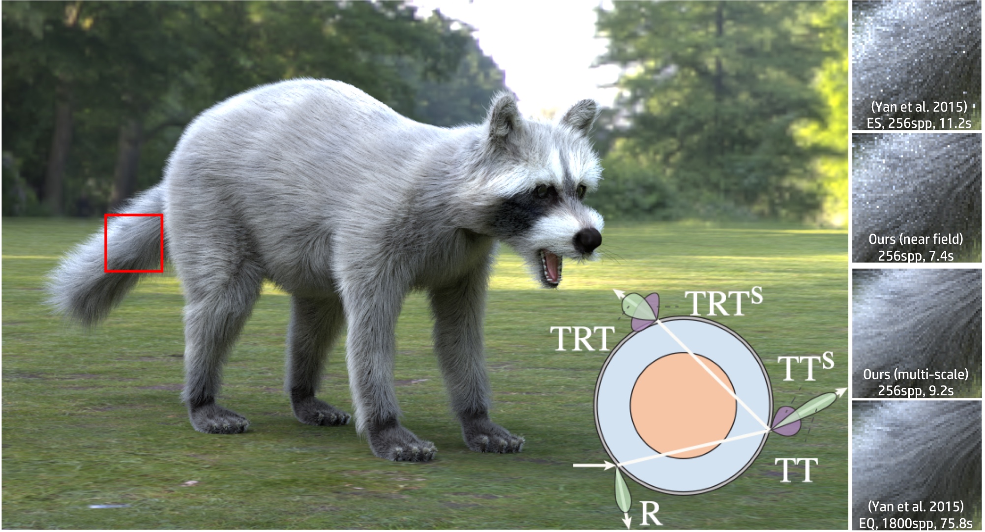
An Efficient and Practical Near and Far Field Fur Reflectance Model
SIGGRAPH 2017
1University of California, Berkeley 2University of California, San Diego
Abstract
Physically-based fur rendering is difficult. Recently, structural differences between hair and fur fibers have been revealed by Yan et al. (2015), who showed that fur fibers have an inner scattering medulla, and developed a double cylinder model. However, fur rendering is still complicated due to the complex scattering paths through the medulla. We develop a number of optimizations that improve efficiency and generality without compromising accuracy, leading to a practical fur reflectance model. We also propose a key contribution to support both near and far-field rendering, and allow smooth transitions between them. Specifically, we derive a compact BCSDF model for fur reflectance with only 5 lobes. Our model unifies hair and fur rendering, making it easy to implement within standard hair rendering software, since we keep the traditional R, TTs, and TRTs lobes in hair, and only add two extensions to scattered lobes, TTs and TRTs. Moreover, we introduce a compression scheme using tensor decomposition to dramatically reduce the precomputed data storage for scattered lobes to only 150 KB, with minimal loss of accuracy. By exploiting piecewise analytic integration, our method further enables a multi-scale rendering scheme that transitions between near and far field rendering smoothly and efficiently for the first time, leading to 68X speed up over previous work.Download
PaperCode
Video
Database
1. Visualization Raw Reflectance data
Here is the visualization of the fitted reflectance data.
Each link is a .txt file containing lines in the following format:
phi theta value
where theta and phi are longitudinal and azimuthal incident angles, respectively. Note that, both theta and phi are using coordinates of the gantry, where theta in [40, 80] maps to [50, 10] degrees and phi in [70, 290] maps to [-20, 200] degrees, following the notations in our paper. The previous work contains the measured data.
The plots show logarithm values.
| Bobcat | 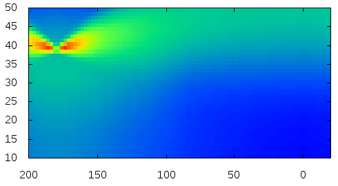 |
Cat | 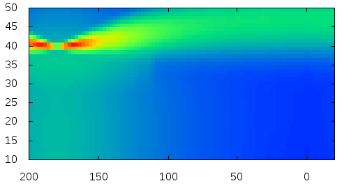 |
| Deer | 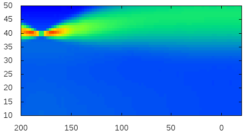 |
Dog | 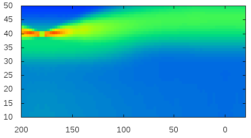 |
| Human | 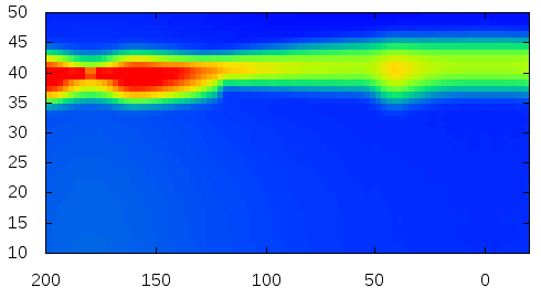 |
Mouse | 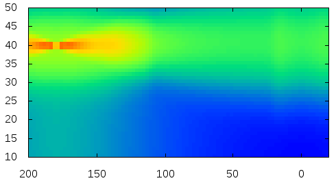 |
| Raccoon | 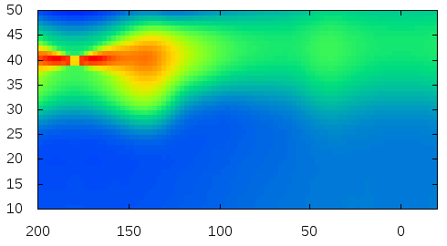 |
Sprningbok | 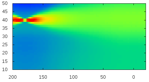 |
| Rabbit | 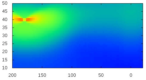 |
2. Compressed Precomputed Scattering Profiles CN and CM
Both CN and CM are 1D profiles for 3D sets of parameters, so they are essentially 4D tables. We provide the compressed pre-computed data here:
The precomputed longitudinal and azimuthal scattering profiles CM and CN are 4D tensors. We refer to tensor decomposition techniques to compress them. Here is a code snippet showing how to read the compressed scattering profiles and how to perform the tensor decomposition. The code should be very easy to understand.
// Number of bins
#define NUM_SCATTERING_INNER 24
#define NUM_H 16
#define NUM_G 16
#define NUM_BINS 720
#define NUM_THETA 16
// Storage
float scattered[NUM_SCATTERING_INNER][NUM_H][NUM_G][NUM_BINS];
float scatteredDist[NUM_SCATTERING_INNER][NUM_H][NUM_G][NUM_BINS];
float scatteredM[NUM_SCATTERING_INNER][NUM_THETA][NUM_G][NUM_BINS];
void initialize(const char *medullaFilename) {
size_t bytesRead;
// Read compressed scattering profiles.
FILE *fp = fopen(medullaFilename, "rb");
if (!fp) {
printf("Can't read precomputed scattering profiles!\n");
return;
}
// Azimuthal
float n1_lambda[16];
float n1_u0[23][16];
float n1_u1[16][16];
float n1_u2[16][16];
float n1_u3[720][16];
bytesRead = fread(n1_lambda, sizeof (float), 16, fp);
bytesRead = fread(n1_u0, sizeof (float), 23 * 16, fp);
bytesRead = fread(n1_u1, sizeof (float), 16 * 16, fp);
bytesRead = fread(n1_u2, sizeof (float), 16 * 16, fp);
bytesRead = fread(n1_u3, sizeof (float), 720 * 16, fp);
// Azimuthal Dist
float n2_lambda[16];
float n2_u0[23][16];
float n2_u1[16][16];
float n2_u2[16][16];
float n2_u3[720][16];
bytesRead = fread(n2_lambda, sizeof (float), 16, fp);
bytesRead = fread(n2_u0, sizeof (float), 23 * 16, fp);
bytesRead = fread(n2_u1, sizeof (float), 16 * 16, fp);
bytesRead = fread(n2_u2, sizeof (float), 16 * 16, fp);
bytesRead = fread(n2_u3, sizeof (float), 720 * 16, fp);
// Longitudinal (backward)
float m1_lambda[16];
float m1_u0[16][16];
float m1_u1[16][16];
float m1_u2[16][16];
float m1_u3[360][16];
bytesRead = fread(m1_lambda, sizeof (float), 16, fp);
bytesRead = fread(m1_u0, sizeof (float), 16 * 16, fp);
bytesRead = fread(m1_u1, sizeof (float), 16 * 16, fp);
bytesRead = fread(m1_u2, sizeof (float), 16 * 16, fp);
bytesRead = fread(m1_u3, sizeof (float), 360 * 16, fp);
// Longitudinal (backward)
float m2_lambda[16];
float m2_u0[16][16];
float m2_u1[16][16];
float m2_u2[16][16];
float m2_u3[359][16];
bytesRead = fread(m2_lambda, sizeof (float), 16, fp);
bytesRead = fread(m2_u0, sizeof (float), 16 * 16, fp);
bytesRead = fread(m2_u1, sizeof (float), 16 * 16, fp);
bytesRead = fread(m2_u2, sizeof (float), 16 * 16, fp);
bytesRead = fread(m2_u3, sizeof (float), 359 * 16, fp);
fclose(fp);
// Reconstruct the actual scattering profiles.
memset(scattered, 0, sizeof (float) * NUM_SCATTERING_INNER * NUM_H * NUM_G * NUM_BINS);
memset(scatteredDist, 0, sizeof (float) * NUM_SCATTERING_INNER * NUM_H * NUM_G * NUM_BINS);
memset(scatteredM, 0, sizeof (float) * 16 * NUM_THETA * NUM_G * NUM_BINS);
for (int i = 1; i < NUM_SCATTERING_INNER; i++)
for (int j = 0; j < NUM_H; j++)
for (int k = 0; k < NUM_G; k++)
for (int l = 0; l < NUM_BINS; l++)
for (int t = 0; t < 16; t++) {
scattered[i][j][k][l] += n1_lambda[t] * n1_u0[i - 1][t] * n1_u1[j][t] * n1_u2[k][t] * n1_u3[l][t];
scatteredDist[i][j][k][l] += n2_lambda[t] * n2_u0[i - 1][t] * n2_u1[j][t] * n2_u2[k][t] * n2_u3[l][t];
}
for (int i = 0; i < 16; i++)
for (int j = 0; j < NUM_THETA; j++)
for (int k = 0; k < NUM_G; k++) {
for (int l = 0; l < NUM_BINS / 2; l++)
for (int t = 0; t < 16; t++)
scatteredM[i][j][k][l] += m1_lambda[t] * m1_u0[i][t] * m1_u1[j][t] * m1_u2[k][t] * m1_u3[l][t];
for (int l = 0; l < NUM_BINS / 2 - 1; l++)
for (int t = 0; t < 16; t++)
scatteredM[i][j][k][l + NUM_BINS / 2 + 1] += m2_lambda[t] * m2_u0[i][t] * m2_u1[j][t] * m2_u2[k][t] * m2_u3[l][t];
}
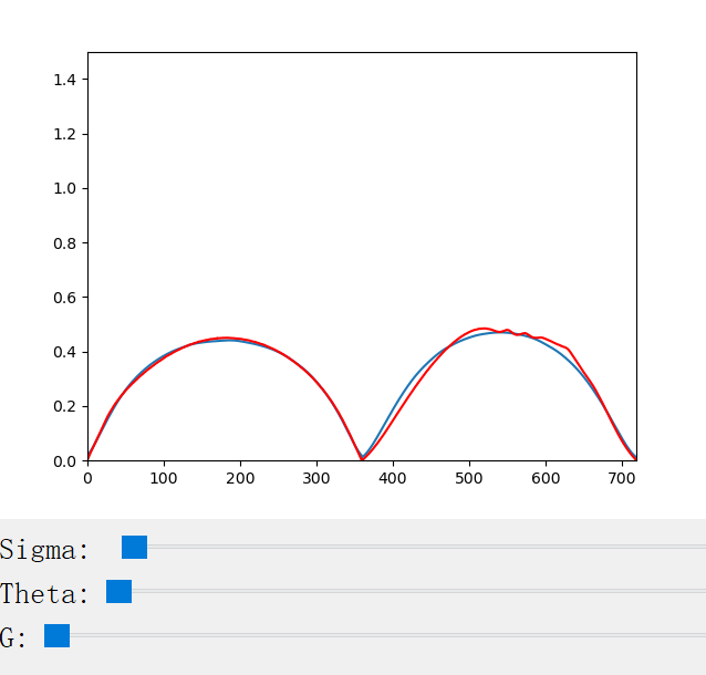
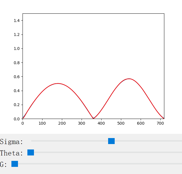
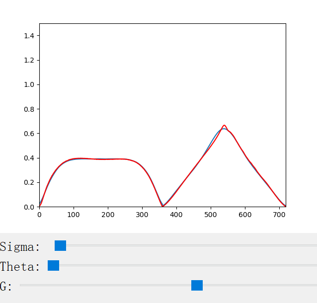
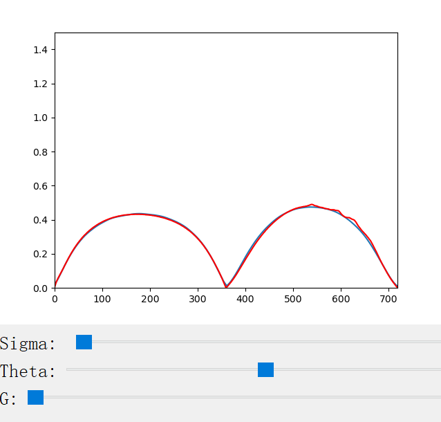
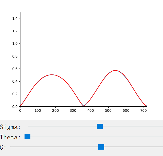
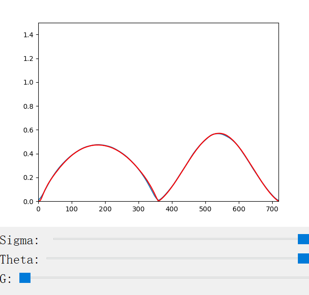
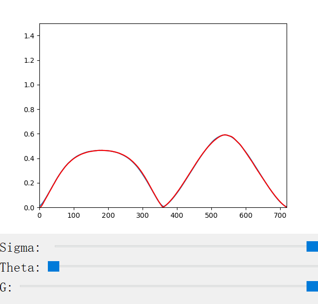
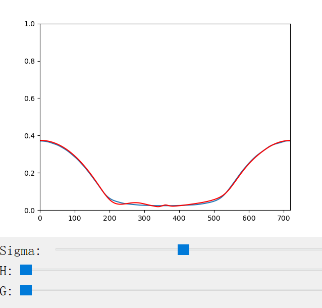
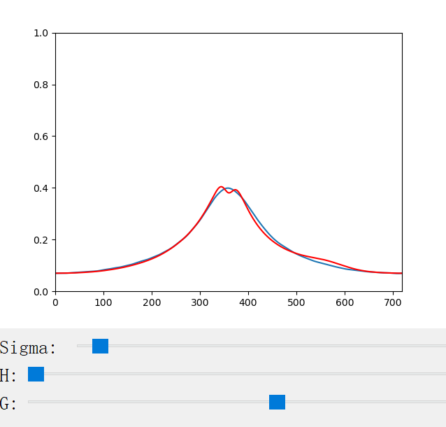
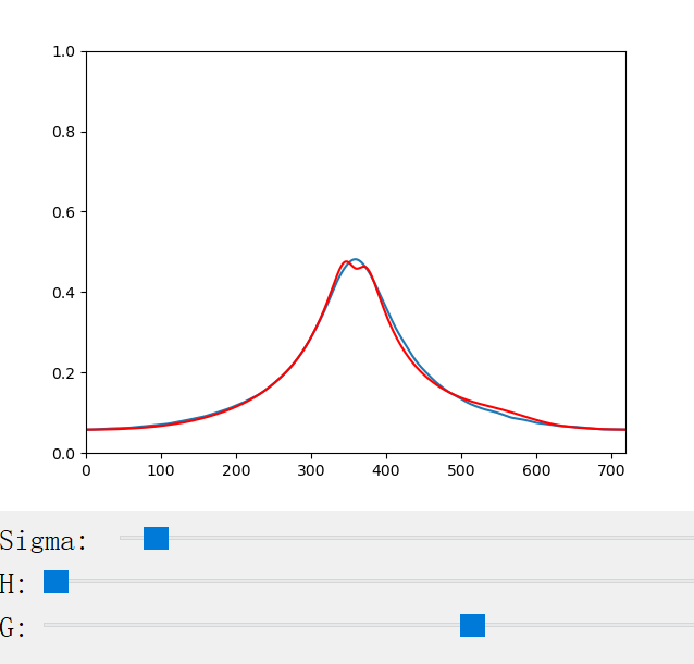
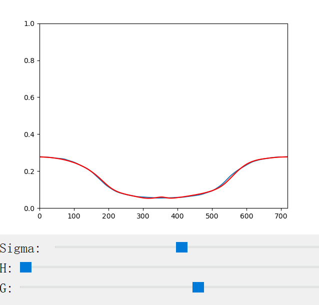
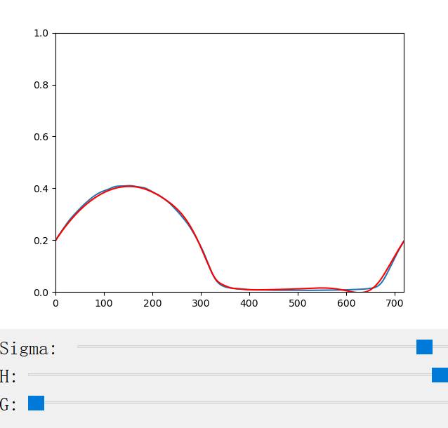
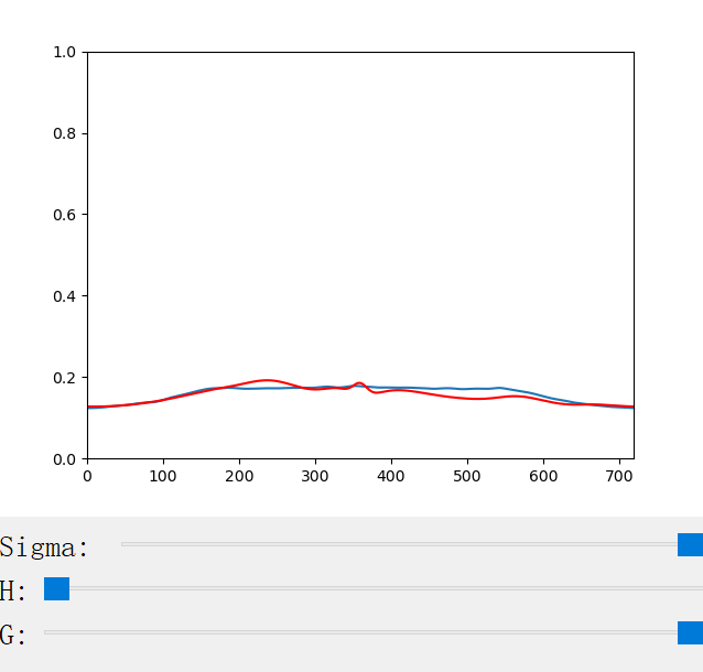
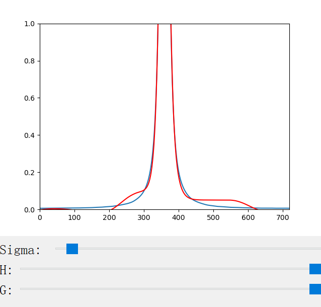
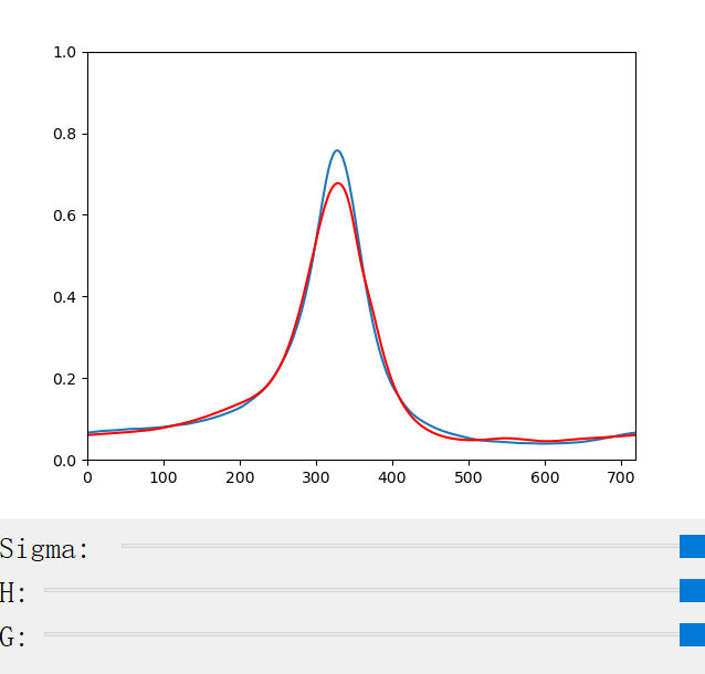
}3. Visualization of Scattering Profiles CN and CM
The scattering coefficient changes with the scattering coefficient σ, the anisotropy factor g, the azimuthal offset h (for CM only), and the longitudinal incident angle θ (for CN only). We provide a handy python program for the visualization of the scattering profiles:
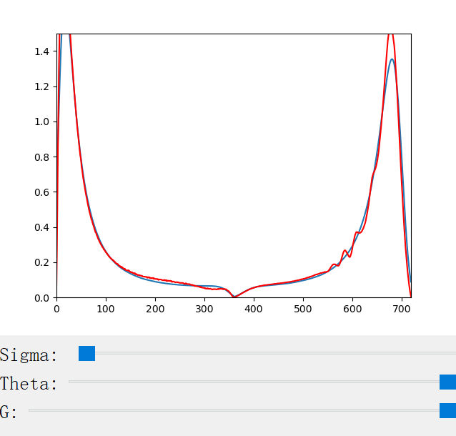
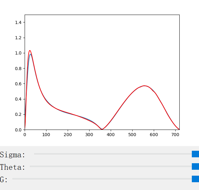
The following figures show the scattering profiles of CN.
 |
 |
 |
 |
 |
 |
 |
 |
 |
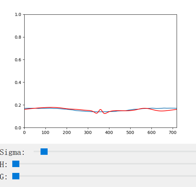
The following figures show the scattering profiles of CM.
 |
 |
 |
 |
 |
 |
 |
 |
 |
Bibtex
 @article{yan2017efficient,
  title={An Efficient and Practical Near and Far Field Fur Reflectance Model},
  author={Yan, Ling-Qi and Jensen, Henrik Wann and Ramamoorthi, Ravi},
  journal={ACM Transactions on Graphics (Proceedings of SIGGRAPH 2017)},
  year={2017},
  volume={36},
  number={4},
}